Home
Welcome to the website hosting the lecture materials for The University of Manchester’s COMP60261 (Secure Computer Architecture and Systems), Part 1. You can use the menu on the left to navigate the materials: for each lecture, you can access the lecture notes as well as the lecture slides.
The lecture slides for Part 2 of the course are available on Canvas.
Instructor: Pierre Olivier
Logistics
You can access the slides 🖼️ for this lecture.
Unit Organisation
COMP60261 is divided into two main parts:
Part 1: Systems Software Security. This part runs for the first 6 weeks of the semester. The instructor is Dr. Pierre Olivier.
Part 2: Hardware Security. This part runs for 5 weeks after Part 1. The instructor is Prof. John Goodacre.
The last week of the semester (the last week of Part 2) will also include an exam preparation session.
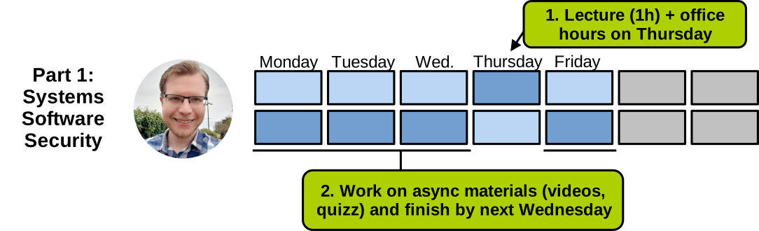
The learning content for each part of the course unit is delivered slightly differently. Part 1 (first 6 weeks, with Pierre) follows a blended learning approach: there is a 1-hour live session (lecture) slot per week, and after that session you’ll need to work on a series of asynchronous materials: lecture videos, and quizzes. The videos represent additional lecture materials not covered during the live sessions, and watching them is mandatory to succeed in the course unit. Please watch the videos for a particular week after the corresponding live session, and furthermore make sure to watch them before the live session of the subsequent week. Part 1’s per-week organisation can be illustrated as follows:
Part 2 follows a more traditional organisation, with a 2-hour live session (lecture) and a quiz to complete after that session each week:
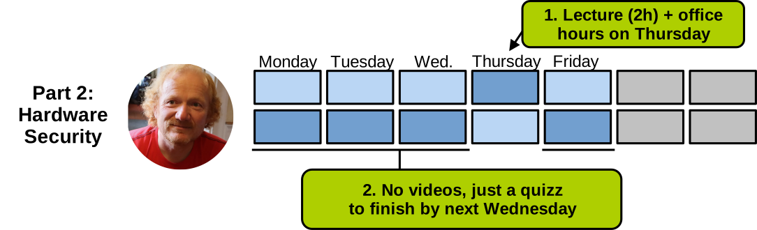
For both parts, the instructor will also hold 1 hour of office hours per week.
Assessment
The summative (i.e., marked) assessment for the unit is divided into:
- Coursework: lab exercises (30% of the final mark): there are a total of 4 lab exercises to be done throughout the semester.
- Final exam (70% of the final mark): taken at the end of the semester.
Each lab exercise counts for 25% of the coursework mark. You should start working on each exercise at least 2 weeks before the deadline.
The weekly quizzes are formative (i.e., not marked). Although they are not marked, it is important to complete them each week, as they allow you to confirm that you understand the content learnt through the lecture materials. These quizzes are also an excellent way to practise for the final exam.
COMP60261 Canvas Page
The unit has a page on Canvas.
Everything regarding the course can be accessed from that Canvas page:
- Schedule (what to do each week)
- Lecture recordings, videos, slides
- Quizzes
- Lab exercise briefs
- Discussion boards
- Reading list
Required Software Setup
All programming exercises should be done in a Linux x86-64 (Intel/AMD CPU) environment. To bring up such an environment, there are several solutions, listed on the “required setup” page of the first lab exercise here. Please make sure you have your setup up and running (e.g., a VM installed and up and running) by the end of the first week of teaching, because lab exercises start in the second week.
Code Snippets in Lecture Materials
The slides used in the live lectures and videos (Part 1) are available on Canvas. They are interactive: when watching the videos or attending the lectures, you are encouraged to access them for clickable links and to try out the code discussed on many slides. Here is an example of a code snippet embedded in the slides (a ‘hello world’ in C):
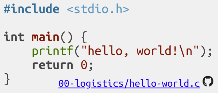
You can click on the blue link at the bottom right of the snippet to download the corresponding source code, so you can build and run the resulting program on your computer if you have a native or virtualised Linux x86-64 setup. If you do not have such a setup (e.g., MacBooks with ARM CPUs), you can also click on the GitHub icon at the bottom right to access a GitHub repository holding all the code snippets presented in the lectures. That repository can be loaded into a GitHub Codespace, allowing you to build and run the program in your browser, independently of your computer/CPU architecture. To find a particular snippet, follow the path in the repository indicated by the blue link at the bottom right of that snippet. Instructions on how to build and run C programs will be given during the first week of teaching.
Contact Information: How to Get Help?
If you have any questions regarding the unit, in increasing order of urgency:
- Step 1: come to the next support session;
- Step 2: use the discussion boards on Canvas, the instructors are generally quite responsive;
- Do not post answers there, or your post will be deleted.
- Step 3, only if urgent: contact the instructor by email (contact information is available on Canvas).
Core Concepts
You can access the slides 🖼️ for this lecture.
Computer Security
Computer security has been historically focused on protecting physical machines to prevent theft of or damage to the hardware. Today, in many scenarios the value of the data that is processed, stored, and exchanged by computers is greater than that of the hardware itself. Thus, modern computer systems security focuses on information security: the key ideas are to prevent theft of or damage to the information handled by the computer, and to prevent disruption of the various services provided by computer systems. In other words, systems security aims to safeguard computer systems against unauthorised 1) access, 2) modification, and 3) disruption.
Computer systems security can be broken down into these two main components:
- Software security: protecting applications and systems software against vulnerabilities and their exploitation; and
- Hardware security: protecting CPU/memory/devices against attacks.
Software and hardware security are heavily intertwined: the software relies upon hardware features to enforce various kinds of software-level security policies and invariants. To that end, the software controls the hardware and makes a series of assumptions that it behaves correctly. There are also many forms of attacks that cross the software-hardware boundary.
On the software side, systems security is concerned with the safety of systems software. Systems software comprises various types of low-level software that manipulate the hardware directly, or that are at least considered close to the hardware: these include operating systems, virtual machine monitors and other virtualisation technologies, and low-level applications such as language runtimes/interpreters, web servers, system utilities, etc.
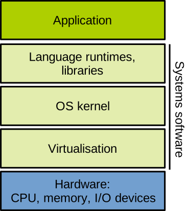
We are going to see a lot of such stacked diagrams in this unit. A computer system can be represented as a stack of layers: the hardware (CPU/memory/devices) is at the bottom, and the software on top of it. The software itself is a pile of stacked layers of abstractions, with the low-level components (those manipulating the hardware more or less directly) such as the OS kernel or a virtual machine monitor at the bottom, and higher level components (applications and libraries) executing on top. The idea is that a high-level layer generally needs to go through the stack to access the lower-level components: for example, applications rarely invoke the operating system directly, but rather make use of libraries to do so. Applications don’t access the hardware directly either, but must request services from the operating system to do so.
Why is Systems Security Important?

On 4th June 1996, the first flight of the European Space Agency’s Ariane 5 rocket took place. 40 seconds after lift-off, the rocket went off track and disintegrated, as shown in the picture above. The root problem was a 16-bit signed integer overflow in a software module. That module integrated code originally written for Ariane 4, the previous generation’s rocket. That code made assumptions that no longer held for Ariane 5, which led to the overflow and ultimately the destruction of the rocket. It was not even doing anything useful after lift-off, so one may ask why it was even running. The total cost of the incident (i.e., of the bug) was $370 million.
Beyond this particular incident, today our world is massively computerised, and the impact of cyberattacks is huge: critical service disruption, financial losses, theft and destruction of critical and personal data, etc. In 2017, private records from more than 160 million US and UK citizens were stolen from the Equifax credit reporting agency following a cyberattack. The lawsuits that followed led to Equifax having to pay up to $700 million in settlement. In 2024, a cyberattack on London hospitals affected more than 800 planned operations and 700 outpatient appointments, requiring them all to be rescheduled.
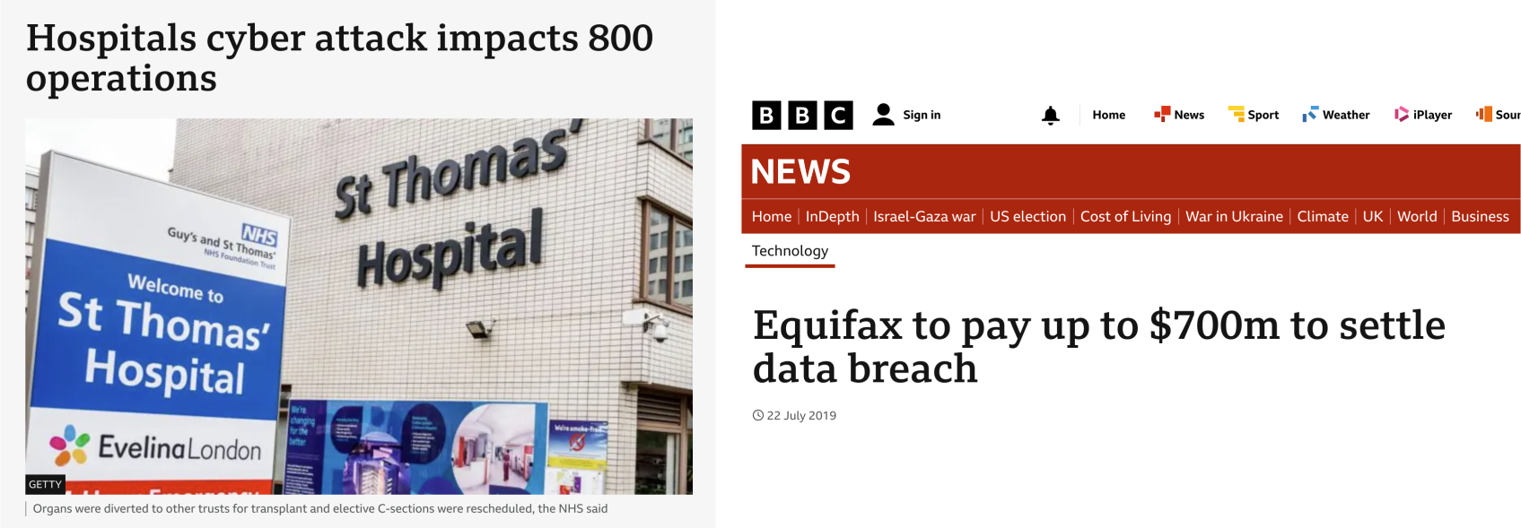
These are just a few examples of how bad things can be, and the problems illustrated here are made even more concerning as computer systems are increasing in complexity, so the likelihood of vulnerabilities that enable cyber incidents and attacks is increasing, and the threats/attack vectors are constantly evolving.
Attack Surface
Computer systems are not perfect and programmers implementing them make mistakes and introduce bugs. Some of these bugs represent security vulnerabilities that can be exploited to mount attacks with various effects on the system integrating the buggy and vulnerable software/hardware component. Vulnerabilities can be present at every level of the hardware/software stack:
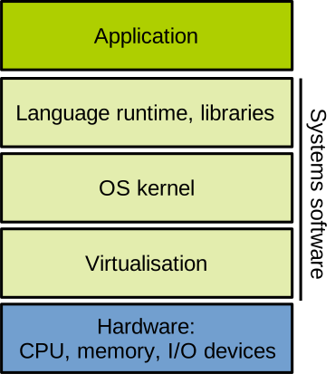
At the application level, any bug that can be triggered by external input (e.g., network, command line arguments, etc.) that may be under the control of an attacker represents a potential security issue. Taking our previous example, the Equifax breach, the attack was made possible because of a bug in Apache Struts: CVE-2017-5638 was a vulnerability in a web application parser allowing an attacker to execute code remotely and completely take over the server hosting the web application.
Vulnerabilities in commonly used software are classified and referenced as Common Vulnerabilities and Exposures (CVEs): each identified security issue gets its own number made up of the year it was discovered and an identifier.
Going down the stack, vulnerabilities can also be present in libraries and language runtimes that are used to run most applications.
A very serious example here is the 2018 NodeJS event-stream attack.
An attacker took over the event-stream library repository, and released a malicious version of the library, designed to steal from crypto wallet software.
The attack was widespread as event-stream was used extensively (~100 million downloads that year).
Further down the stack, the operating system is a cornerstone of security in a computer system, because it executes with a high level of privilege, so an attacker taking over an OS or making that OS misbehave can do a lot of damage. Operating systems are also, in most cases, huge and complicated pieces of software, implemented with millions or tens of millions of lines of code: the chances of these gigantic codebases containing bugs are very high. A famous example of an OS vulnerability is Linux’s CVE-2016-5195 (Dirty CoW): to exploit it, a normal (non-root) user triggers a race condition to obtain write access to read-only memory mappings and escalate privileges to become the administrator (root). This was used to, among other things, root Android phones.
Virtualisation software suffers from the same issues as the OS layer: it is complex software that runs with elevated privileges. The Xen virtual machine monitor suffered in 2014 from CVE-2014-7188, which is a read overflow in the interrupt controller emulation, allowing code running in an unprivileged virtual machine to leak data from the virtual machine monitor or from other virtual machines running on the same host. Imagine an attacker renting a cloud VM, able to steal critical data from either the other tenants running on the same physical machine or the cloud provider. The patch to fix the issue required an emergency forced reboot of about 10% of Amazon Web Services’ Elastic Cloud (AWS’s VM renting offering), which was a severe interruption of service.
Finally, at the bottom of the stack, the hardware is often assumed to work perfectly by computer system developers working on the software stack. Unfortunately the hardware is not exempt from bugs and vulnerabilities. In 2017, the Spectre and Meltdown vulnerabilities were discovered by researchers. These vulnerabilities allow an attacker to leak data between processes or from the kernel by exploiting the speculative execution engine of Intel processors. The speculative execution feature of modern processors can be tricked into leaking data from processes and the kernel. Some countermeasures were developed in software and through CPU microcode updates, but they introduced non-negligible performance slowdowns.
Vulnerabilities
As said above, modern software and hardware used in production are increasingly complex. The Linux kernel v6.12 is made up of 26 million lines of (mostly C) code. An Apple Silicon M3 Max SoC has 92 billion transistors. Given the scale and complexity of these components, there is simply no way to prove that they are 100% correct and bug-free.
In fact, they are likely not correct and bug-free: software/hardware designers and engineers are human; they make mistakes and introduce bugs. Many bugs are mostly silent under normal operation, so they are hard to detect, and may live for years in codebases without being identified. These bugs have various consequences: obviously they can lead to software/hardware instability or crashes, which is already bad enough (see the Ariane 5 issue mentioned above). Furthermore, some bugs, when triggered in a certain way, will allow an attacker to cause harm to the computer system integrating the buggy software/hardware component: these are vulnerabilities.
Attacker’s Objectives
A malicious actor attacking a computer system may want to:
- Read what they are not supposed to read: sensitive data such as passwords or crypto keys, information about the target system (e.g., open ports) to enable further attacks, etc.
- Write what they are not supposed to write: corrupt sensitive data structures to escalate privilege, inject malicious code and data, forge access tokens, escape detection, etc.
- Control what they are not supposed to control: disturb operation (denial of service), execute code to enable further attacks, etc.
Defender’s Objectives: The CIA Triad
On the defence side, these are the high-level security properties we want computer systems to maintain:
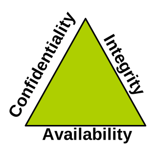
- Confidentiality: preventing unauthorised disclosure of sensitive information. Examples of confidentiality enforcement include using encryption, access control, secure deletion, etc.
- Integrity: preventing unauthorised tampering with sensitive information. Examples include using checksum verification, digital signatures (keys), etc.
- Availability: preventing disturbances to the operation of a computer system, for example with denial of service protection, redundancy/replication, backups, etc.
Another important concept is that of identity, i.e., making sure that an actor is who they claim to be. This can be achieved by using passwords, certificates, and other identification methods.
Trust Models
When protecting a computer system, establishing trust models means reasoning about what components of the system are trusted to work correctly vs. what components are not. Taking the point of view of the different actors that may interact with a particular computer system, the trust model will vary. Here is an example in the context of Infrastructure as a Service (IaaS, i.e., the renting of virtual machines – VMs – in the cloud). We can represent the system as follows:
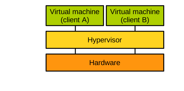
A cloud provider is offering virtual machines (VMs) for rent to clients (also called tenants). The cloud provider owns the host hardware, and uses a virtual machine monitor (also called hypervisor) to multiplex the hardware between these VMs. Each tenant gets their own VM. From a high-level point of view, the cloud provider does not trust the tenants: they may run arbitrary, possibly malicious, software within their VM. The tenants trust the cloud provider to provide a working service, but tenants do not trust each other: for example, two competing companies may end up renting 2 VMs located on the same host, and company A does not want its data to be accessed by company B – even if it is located on the same physical host.
From the cloud provider’s point of view, the trust model is as follows:
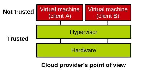
The hardware and the hypervisor are trusted to work correctly. The hypervisor enforces the isolation between VMs, and as mentioned, we do not want one VM being able to access the memory of another. The hypervisor must also enforce the isolation between VMs and itself: this is important because in most virtualisation scenarios the hypervisor has access to the memory of the entire machine, i.e., the memory of all VMs, and we do not want a VM to force the hypervisor to access the memory of another VM on its behalf. The VM/hypervisor isolation is controlled by the hypervisor and enforced through hardware mechanisms, so both entities need to be trusted to work correctly: if that is not the case, the system is not secure.
From the point of view of a tenant (e.g., A), the trust model is the following:
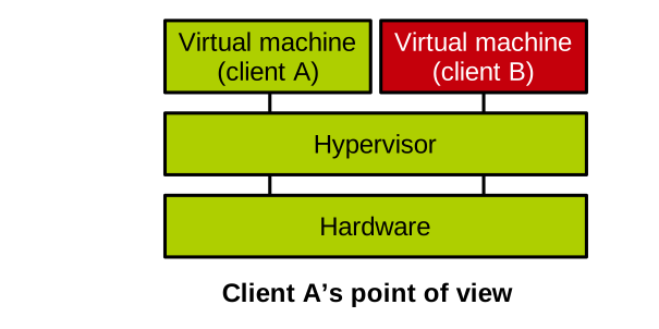
Tenant A does not trust the software running in the VM rented by tenant B. A does trust that the hardware and hypervisor work correctly; otherwise, as described above, nothing would prevent the other tenant, B, from accessing or disturbing A’s VM. From B’s point of view, the trust model is similar: B does not trust A’s VM, but it trusts the hypervisor and the hardware.
Through that example, we can see that trust models vary depending on which actor and scenario are considered.
Trusted Computing Base
The trusted computing base (TCB) is the set of software and hardware components that are critical to the security of the system: they are assumed to be working correctly to maintain the target security guarantees. TCBs are the components shown in green in the picture illustrating our examples of trust models. The TCB should always be as minimal as possible to make it easy to secure: the more software/hardware we need to trust, the greater the chance that the TCB contains bugs/vulnerabilities, and the less likely our trust model is to hold. The TCB should also always be isolated from non-critical components of the system: they are not trusted, and if their interactions with the TCB are not controlled, the security of the system is at risk. In our IaaS example, from the cloud provider’s point of view, the TCB includes the hardware and host systems software (hypervisor, host kernel/firmware/boot process).
Threat Model
When reasoning about a system to secure/defend, in addition to establishing at least one trust model and defining the corresponding trusted computing base, security practitioners must also establish a threat model. It represents a series of assumptions about what the attacker can and cannot do.
Next, we discuss a few examples of threat models within the context of our IaaS scenario.
Attacks always come from untrusted system components and are aimed at trusted components. If we first take the point of view of the cloud provider and consider the relevant trust model, our threat model is as follows:
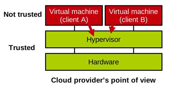
The provider does not trust the tenants, so this is where attacks come from. Tenants may attempt to exploit the interface exposed by the virtual machine monitor to trigger bugs at that level and disturb or access the memory of other tenants or the hypervisor. Tenants may also attempt to leverage hardware vulnerabilities (e.g., side channels) to achieve these goals.
From tenant A’s point of view, we have the following threat model:
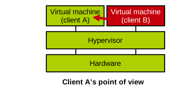
A does not trust B, which is where attacks come from. In addition to B attacking the hypervisor or the hardware to get to A, as explained in our scenario from the cloud provider’s point of view, B may also try to subvert A, assuming the two virtual machines interact somehow.
If we now take the point of view of tenant B, let us, for the sake of illustration, consider a trust model that is slightly different from the one seen above. In that trust model, B does not trust A, but it also does not trust the virtual machine monitor:
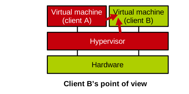
That is a viable trust model: many companies are reluctant to use the cloud to offload some of their internal IT workloads because they fear the cloud provider having access to their business data. With that trust model, our threat model is as follows: attacks can come from A, but also from the hypervisor. That is a particularly difficult threat model to protect against, because the hypervisor runs on the CPU at a higher privilege level than B’s VM. Still, there are some modern hardware mechanisms that allow preserving B’s VM confidentiality even in the presence of an untrusted hypervisor: they are called trusted execution environments, and we will cover them in a future lecture.
Isolation Approaches
We have seen that to protect a system and enforce a trust model, trusted components need to be isolated from untrusted components: in our example, the hypervisor must be isolated from VMs, a particular VM needs to be isolated from the other VMs running on the same host, etc.
There are three high-level isolation models, corresponding to three trust models:
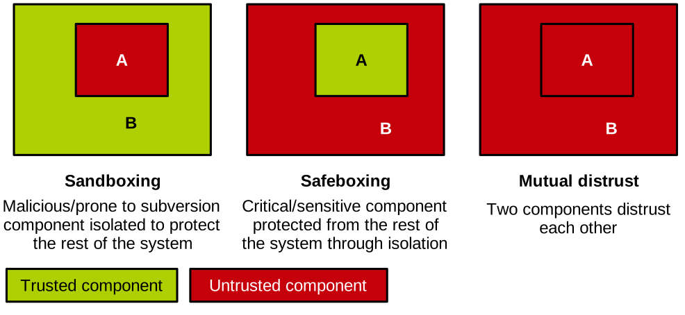
Sandboxing an untrusted component means isolating it from the (trusted) rest of the system. Sandboxing is applied to components with a low degree of trust, prone to being subverted: third-party software, code written in unsafe languages, etc. This approach is quite widespread in today’s computer systems: a process is isolated from the rest of the system by the operating system. Similarly, a VM is isolated from the rest of the system by the hypervisor. Taking a different example, web pages belonging to different sites and running in different tabs are sandboxed in a web browser. The web browser also sandboxes the execution of untrusted code such as JavaScript.
Safeboxing a trusted component corresponds to isolating it from the (untrusted) rest of the system. Safeboxing is applied to components that are particularly critical to the security of a system: the TCB or part of it, as well as components manipulating critical data. The approach can, for example, be used to isolate a crypto library in a web browser, or code manipulating cleartext passwords in memory in the context of a password check.
Finally, mutual distrust corresponds to the isolation of components that distrust each other. There are many examples of mutual distrust scenarios: peers communicating within a peer-to-peer network, a web browser and an HTTP server exchanging requests and web pages over a network connection, different processes communicating through inter-process communication, and our past example of a VM interacting with an untrusted hypervisor.
The Principle of Least Privilege
The principle of least privilege states that each component (processes, users, etc.) in a system should only be granted the minimum permissions required to perform its duties correctly. This limits the damage that can be done to the system should this component be subverted by an attacker. This principle was introduced in the paper The Protection of Information in Computer Systems in 1975 by Saltzer and Schroeder. This is a seminal paper in the field of computer systems security, well worth reading.
The principle of least privilege is applied extensively today, and examples are plentiful:
- The privilege levels of execution on modern CPUs prevent standard applications from executing privileged instructions (e.g., the ability to map memory or to shut down the computer), reserving that privilege to the operating system only.
- Many computer systems manage permissions with access control techniques, such as user-based file access permissions, application permissions (to access the camera, microphone, location, etc.) on mobile systems, etc.
- The program
sudo, that is supposed to be used only for the operations requiring root privileges - etc.
The principle of least privilege is an ideal objective that we try to approach as much as possible when securing a computer system. In practice, it is hard, not to say impossible, to fully achieve it: for reasons of complexity or performance, system components often end up overprivileged.
Introduction to C
You can access the slides 🖼️ for this lecture.
Here we will briefly introduce the C programming language. The vast majority of systems software is written either in C or in C++, which is an extension of C. These languages are also known to be memory-unsafe, a concept we will study in detail in this unit and that has very important implications in terms of security. For these reasons, knowledge of C programming is quite important in systems security.
This is a short introduction covering the basics of the language, its standard library, pointers, and memory management. Readers already familiar with these areas can skip this part. For readers with absolutely no knowledge of the language, this will not be a comprehensive overview of C, so make sure to check the recommended additional readings available on Canvas.
The C Programming Language
C is a very old programming language. It was designed in the 70s, but it is still widely popular today. In fact, it is one of the top 10 programming languages in most popularity rankings. There are many popular programs written in C:

C is the default programming language for systems software: operating systems (e.g., Linux or macOS), web servers (Apache, Nginx, etc.), database systems (e.g., SQLite), virtual machine monitors (e.g., Xen). Many language runtimes such as Perl or Python are written in C, as well as other tools that programmers use daily, for example Git.
There are many reasons why C is still a popular programming language. First, it is low-level and lets the programmer manipulate hardware, such as the CPU or memory, quite directly. This is convenient when writing low-level software such as operating systems. Second, because of the simplicity of the language, programs written in C can be very fast and can have a very low memory footprint: this is crucial in domains such as high-performance computing and embedded systems. C has also established a popular syntax, which is reused by many languages that came afterwards, such as Java, C++, and many others. Finally, C is portable: you will find compilers translating C code for each modern CPU architecture.
All these benefits come at a cost: C leaves a lot of room for the programmer to make mistakes, in particular when manipulating memory. We say that C lacks memory safety, and the bugs that can be introduced this way can lead to serious security issues, as we will see later in this unit.
Despite these problems, C is still extensively used in many domains even beyond systems software: HPC, embedded systems/IoT, etc.
Hello World in C
This is the traditional “hello, world” program, written in C:
#include <stdio.h> // needed to use printf which is declared in stdio.h

// main is the program entry point
int main() {
    printf("hello, world!\n"); // print "hello, world!" on the console
    return 0;                  // returning from main exits the program
}
The program starts by including stdio.h, which is part of the standard library and will give us access to a function to print text to the console.
Then we have the definition of the main function: it returns an integer (int) and does not take any parameters.
In C main is the entry point, which means it contains the code that will run when the program starts.
Within main we use the printf function to print "hello, world!" to the console.
As you can see, every statement in C ends with a semicolon: ;.
The program returns 0 from main.
0 is an integer code that, as a convention, means success in C.
Returning from the main function will also exit the program.
C is a compiled language, which means we first need to transform our source code, which is nothing more than a text file, into an executable program that can be run:
$ gcc hello.c -o hello
$ ./hello
hello, world!
We compile on the command line with GCC, a C compiler.
It takes the source file as input, here it is hello.c.
Then we have -o and the name of the executable we want to create, here it is hello.
Once the compiler is done, the program can be executed by simply typing ./hello.
Warning and Errors. Another important aspect of the compiler is that it will check for programming mistakes and will emit warnings and errors. These will be displayed on the console. Errors are unrecoverable and will stop the compilation process, while warnings are not. Make sure to fix warnings and errors in the order they are emitted by the compiler. Please also make sure that all the code you produce as part of this unit compiles without any warning or error.
Variables
In C, like in many languages, variables have a name, a type, and a value.
For example, in the code below, the first variable declared is named a:
#include <stdio.h>

int main() {
  int a;                 // declare a of type int (signed integer)
  int b; int c;          // b and c of type int
  int d = 12;            // declare d of type int, and set its value
  int x, y = 10, z = 11; // declare x, y and z, set values for y and z

  a = 12;      // set a's value to 12
  b = 20;      // set b's value to 20
  c = 10 + 10; // set c's value to 20
  a = b;       // a = 20
  d++;         // d = d + 1
  y *= 2;      // y = y * 2;
}
a’s type is int, which denotes a signed integer, and after the assignment, a’s value is 12.
Each variable must be declared before being used.
This is done as shown in the code snippet, with the type followed by the name of the variable: int a;.
You can also see how to declare a variable and set its value in a single statement (as with d), and how to declare several variables of the same type in a single statement (as with x, y, and z).
Next, in the code snippet, we manipulate these variables, assigning them values.
You can also see a bit of arithmetic; in particular, pay attention to the d++ statement: it corresponds to incrementing d by one.
The next statement, y *= 2, corresponds to multiplying y by 2.
Types
In C types have two main functions. First, they help the compiler check the validity of the operations applied to variables. Second, they define how much memory space should be allocated to store variables. C has 3 basic types: integers, floating-point numbers, and characters:
int my_integer = -12345;
float my_float = 42.5;
char my_char = 'a';
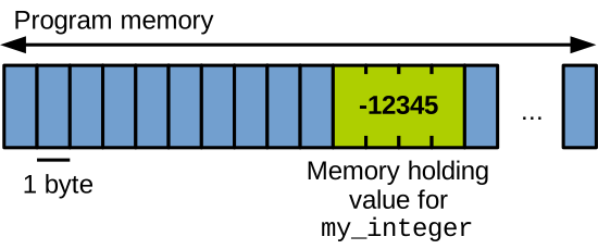
If we look inside the program’s memory at runtime, we’ll see that the compiler reserved a certain amount of space (bytes) for each variable.
For example, here we have my_integer, which is an int (a signed integer).
On an Intel x86-64 CPU an int is stored on 32 bits, which is 4 bytes:
Qualifiers, Storage Size in Memory
Types can be augmented with qualifiers to request more or less space:
int so_short = sizeof(short int);
int so_int = sizeof(int);
int so_uint = sizeof(unsigned int);
int so_long = sizeof(long int);
int so_longlong = sizeof(long long int);
int so_float = sizeof(float);
int so_double = sizeof(double);                           // storage sizes on x86-64:
printf("size of short:         %d bytes\n", so_short);    // 2 bytes
printf("size of int:           %d bytes\n", so_int);      // 4 bytes
printf("size of unsigned int:  %d bytes\n", so_uint);     // 4 bytes
printf("size of long int:      %d bytes\n", so_long);     // 8 bytes
printf("size of long long int: %d bytes\n", so_longlong); // 8 bytes
printf("size of float:         %d bytes\n", so_float);    // 4 bytes
printf("size of double:        %d bytes\n", so_double);   // 8 bytes
Such qualifiers allow storing larger/smaller numbers.
For example, on Intel x86-64, the type short int will be stored on 2 bytes, so it can store fewer signed integers than a traditional int.
Conversely, the type long int will be stored on 64 bits, which is 8 bytes.
float and double are used for floating-point numbers, stored respectively on 4 and 8 bytes on x86-64.
Finally, pay attention to the unsigned qualifier, which lets the programmer indicate that a variable will only store positive integers.
With the qualifiers long/short we can request larger/smaller storage sizes.
The storage size for a given type depends on the architecture, and the programmer should use sizeof to get the exact size of a type on a given machine.
Printing to the Console
As we have seen earlier, the printf function allows us to print text on the console, which is also called the standard output.
It takes as its first parameter what is called a format string, which contains the text to print.
It then takes zero or more additional parameters, which are variable names, referencing the variables whose values should be printed within the format string.
These values replace the special markers located in the format string.
int i = -42;
float f = 12.34;
char c = 'a';
long unsigned int lui = 500;
double d = 42.42;

// prints "-42, 12.34, a, 500, 42.42":
printf("%d, %f, %c, %lu, %lf\n",
    i, f, c, lui, d);
Markers depend on the type of the variable one wants to print.
For example, we use %d for signed integers, %f for floats, and %c for characters.
Markers for types corresponding to numbers can be prefixed with l to indicate longs and doubles.
You can see a few examples in the code snippet above.
If you run this code, the program will display the value of each variable, separated with a comma.
Arrays
Like most languages, C supports arrays.
You can see here how to declare a one-dimensional integer array named array, and how to set each of its elements to a certain value:
int array[4];  // declare an array with 4 elements of type int
array[0] = 42; // set the elements' content
array[1] = 43;
array[2] = 44;
array[3] = 45;
printf("%d\n", array[2]); // print the 3rd element of the array
Note that array indexes start at 0 in C.
With the printf statement you can also see how to reference a particular array slot to print its value.
C also supports arrays with multiple dimensions: the array named arr2d is a two-dimensional array:
int arr2d[2][2];  // declare a 2-dimensional 2x2 array of ints
arr2d[0][0] = 12; // set the elements' content
arr2d[0][1] = 13;
arr2d[1][0] = 14;
arr2d[1][1] = 15;
See how it is declared, with the size of each dimension indicated between brackets. It can then be indexed with 2 sets of brackets, one for each dimension.
Although there is no string type per se in C, strings are represented as arrays of characters.
See this example with str, which contains the string hi:
char str[3];  // in C, strings are array of characters...
str[0] = 'h';
str[1] = 'i';
str[2] = '\0'; // ... that end with the `\0` termination character
Note that in C, to be valid, a string must end with the character \0, which is the termination character.
Make sure when you declare an array that it has enough space for what you want to store plus the termination character.
An important thing about arrays in C is that they are laid out contiguously in memory. We can illustrate the memory layout of each of the arrays in the code snippets above as follows:

array is an array of integers, so on x86-64 each of its elements will have a size of 4 bytes.
They are laid out in memory one after the other: array[0] first, then array[1], and so on.
Similarly, the integers of the two-dimensional array arr2d are laid out contiguously, dimension by dimension.
Finally, regarding the string str, on every architecture the size of a character is one byte.
So the array str looks as follows in memory: h, then i, then the termination character \0.
Conditionals, Functions
Conditionals.
In C we write conditionals as follows: we start with the if keyword, followed by the condition:
int num = 10;

if (num > 0) {
    printf("Number is positive\n");
} else if (num < 0) {
    printf("Number is negative\n");
} else {
    printf("Number is zero\n");
}
If the condition is true, which in C translates into the condition evaluating to something different from 0, the code coming next within brackets will run.
If the condition is false (in other words, if it evaluates to 0), you can add as many else if statements to evaluate additional conditions.
The code within the brackets of the final else will run if none of the previous conditions evaluated to true.
Another form of conditional is the switch-case statement:
int choice = 1;
switch(choice) {
  case 1:
    printf("choice is 1\n");
    break;
  case 2:
    printf("choice is 2\n");
    break;
  default:
    printf("choice is neither 1 nor 2\n");
}
It allows running code based on the value of what’s in between parentheses after switch, here it is choice.
If the value of choice is 1, the code after case 1 will be executed.
If it is 2, the code after case 2 will be executed.
And if it is anything else, the code after default will run.
Make sure to end each of the pieces of code after case with a break to exit the body of the switch.
Functions.
Regarding functions, here you can see how we define a function named add:
int add(int a, int b) {
    return a + b;
}

int main() {
  int result = add(2, 2);
  printf("2 + 2 = %d\n", result);
}
It takes two integers as parameters, a and b, and returns an integer which is in effect the sum of the two parameters.
You can also see how it is called from the main function, which stores its return value in a variable and prints it.
Loops
The for loop will start with i equal to 0, will iterate until i is no longer inferior to 5, and will increment i after each iteration with i++:
int i;

for (i = 0; i < 5; i++) {
    printf("For loop iteration %d\n", i);
}
The while loop does exactly the same thing, however you just specify a condition between parentheses, which when true will have the iterations continue.
That is why i needs to be incremented manually within the loop’s body:
int i = 0;
while (i < 5) {
    printf("While loop iteration %d\n", i);
    i++;
}
Command Line Parameters
Regarding the command line parameters you can pass to your program, in C they are managed through the arguments of the main function:
int main(int argc, char **argv) { // 'char ** argv' means 'char argv[][]'
    printf("Number of command line arguments: %d\n", argc);

    for(int i = 0; i<argc; i++)
      printf("argument %d: %s\n", i, argv[i]);  // no need for braces when the
                                                // body of the loop is a single line
    return 0;
}
argc is an integer that indicates the number of command line parameters.
Note that the first parameter is always the name of the program being executed, so that number will be at least 1.
argv is an array of strings that contains the values of the command line parameters.
In the example code above, the program iterates over all command line parameters and prints the value of each of them.
Custom Types
You can create your own types with the typedef keyword.
This is useful to alias other types, for example long types with several qualifiers, into a single and easy to write type.
For example, in the code below we can alias long long unsigned int with my_int, which is much shorter to write.
After the typedef, we can use my_int anywhere we would have used long long unsigned int.
typedef long long unsigned int my_int;

// 'my_int' is now equivalent to 'long long unsigned int'

int main(int argc, char **argv) {
    my_int x = 12;
    printf("x is: %llu\n", x);
    return 0;
}
Custom Data Structures
You can create custom data structures by aggregating primitive types.
This is done with the struct keyword.
In the code below we have an example of a custom struct person, which has 3 fields:
- A
name, which is a string (an array of characters) - A
size_in_meters, which is a float - And a
weight_in_grams, which is an int
struct person {
    char name[10];
    float size_in_meters;
    int weight_in_grams;
};

void print_person(struct person p) {
    printf("%s has a size of %f meters and "
        "weights %d grams\n", p.name,
        p.size_in_meters, p.weight_in_grams);
}

int main(int argc, char **argv) {
    struct person p1;
    p1.size_in_meters = 1.6;
    p1.weight_in_grams = 60000;
    strcpy(p1.name, "Julie");
    struct person p2 = {"George", 1.8, 70000};
    print_person(p1);
    print_person(p2);
    return 0;
}
In main we can declare a variable p1 which is of type struct person.
Then we can set a value for each of the fields with the . operator.
We also use strcpy (string copy), from the standard library, in order to set the name to “Julie”, which is much faster than setting each character one by one.
Similarly, we have another variable p2, this one declares and sets values for each of the data structure’s fields with a one-liner.
Next we call the print_person function twice, which is defined above: this function prints the value of each field of a struct person.
Observe how it references each field with the . operator.
Rather than typing struct person each time you want to reference your custom type, you can use a typedef.
Below, after having defined a struct named s_person, we can alias it with typedef into person, which is much simpler to use.
Next we just have to use the type person each time we want to refer to our custom data structure type.
typedef struct s_person {
    /* fields here ... */
};

typedef struct s_person person;

void print_person(person p) { /* ... */}

int main(int argc, char **argv) {
    person p1;
    person p2 = {"George", 1.8, 70000};
    /* ... */
}
The fields of an instance of a custom data structure are laid out in memory contiguously and in order. Assume we have the following code:
struct person {
    char name[10];
    float size_in_meters;
    int weight_in_grams;
};

/* ... */

struct person p1 = /* ... */;
Then p1 will be laid out in memory as follows:

The struct person’s fields are a string, a float, and an int.
They are laid out contiguously in memory, in the order defined in the struct declaration, so on x86-64 we have:
- 10 bytes for the string
name, 1 byte for each character - 4 bytes for the float
size_in_meters - 4 bytes for the int
weight_in_grams
C: Pointers
You can access the slides 🖼️ for this lecture.
Here we will cover a central concept in C: pointers. They allow the programmer to manipulate memory quite directly. We will start by defining what a pointer is, and we’ll see in what scenarios using pointers is required or beneficial.
The Virtual Address Space
As you know, each program running on the CPU accesses memory with load and store instructions. These target memory locations called addresses, and the set of addresses a program can read from and write to is named the virtual address space. It is very large; for Linux on 64-bit processors, it ranges from address 0 to 128 TB. Its size is unrelated to the amount of physical memory present in the machine; in fact, most of these virtual addresses are not mapped to physical memory. Each slot in the address space can hold 1 byte, and is indexed by a unique address:

There is one address space for each program in the system. Address spaces are private, and programs do not see each other’s address spaces.
An address is thus a unique location in memory addressable by the program.
The address of a variable is that of the first byte holding this variable.
You can obtain the address of a variable with the & operator:
int x = 42;

printf("0x%x\n", &x);  // print the address of x in hexadecimal
If we assume the following memory layout:
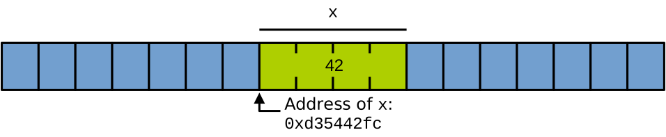
Then, in the example above, the address of x being the address of the first byte holding it, the program will print 0xd35442fc.
Pointers: Definition
Now we can define what a pointer is: a pointer is simply a variable whose value is an address. It can be the address of another variable, or of any other byte of the address space – including parts of the address space containing nothing.
A pointer is declared with the * operator, preceded by the type of the data it references, for example here we have ptr which is a pointer of int, so its type is int *:
int x = 42;
int *ptr = &x;        // ptr is a pointer of int and _points to_ x
printf("%d\n", *ptr); // dereference ptr, print the value of x
ptr holds the address of x; we say that ptr points to x.
A key operation we can realise on a pointer is to access the memory it points to.
This is realised with the * operator; in the code above, we use it to print the value of x through ptr.
The action of accessing the data pointed to by a pointer with the * operator is called dereferencing the pointer.
If we look at how things are laid out in memory we’ll get the following:

Our integer x is located somewhere in memory, and assuming we are on x86-64, its size is 4 bytes.
The address of x is that of the first byte holding it: 0xd35442fc.
When ptr is set to point to x, its value is set to that address, and we can represent this relationship on the diagram with an arrow: ptr points to x.
Notice also that the size of pointers on a given architecture is the width of the memory address bus: 8 bytes on modern 64-bit CPUs.
Now that we know what pointers are, let’s see in what situations they are beneficial.
Passing References Across Functions
Argument Passing in C.
In C, upon a function call, a copy of the arguments is made in memory to create the parameters of the called function.
Check out this example which is a naive attempt at swapping the value of two variables in main:
int swap(int a, int b) {
  int tmp = a;
  a = b;
  b = tmp;
}

int main() {
  x = 10;
  y = 100;
  swap(x, y);
  printf("x=%d, y=%d\n", x, y); // x is still 10 and y is still 100: the swap operated
                               // on a and b in the function swap's stack frame
}
x and y are passed as arguments to swap, which exchanges the values of its parameters a and b.
If we run this program, we’ll see that the values of x and y are unchanged after the function call.
Indeed, when swap was called, the program made copies of the values of x and y for the parameters a and b, swapped the copies’ values, and then discarded these copies as the function swap returned:

Accessing the Calling Context with References.
If we actually want swap to exchange the values of x and y in main’s memory, we need to pass their addresses, and not their values, as parameters:
int swap(int *a, int *b) {
  int tmp = *a;
  *a = *b;
  *b = tmp;
}

int main() {
  x = 10;
  y = 100;
  swap(&x, &y);
  printf("x=%d, y=%d\n", x, y);
}
Here we have updated the function’s parameter types to be pointers to integers, and the swap is now realised on the pointed-to values by dereferencing the pointers.
In main, we no longer pass x and y to the function but rather their addresses, obtained with the & operator.
If you run this program, you will see that the values of x and y are successfully swapped after the call to swap.
What happens is that a copy of the addresses of x and y is created for the pointers a and b.
So we have a pointing to x, and b pointing to y.
By dereferencing these pointers, the swap function is able to update the pointed-to values and perform the swap within the area of memory allocated for the main function:

“Returning” Several Values.
The previous example showed us how pointers can be used to let a function manipulate its calling context.
This is useful in several scenarios, for example you need pointers when you want a function to transmit back to its calling context (i.e., “return”) more than a single value, or to return complex data structures or arrays.
We can study an example here, with the multiply_and_divide function taking 2 numbers n1 and n2 as parameters.
We want this function to “return” three things:
- The product of
n1byn2 - The result of the division of
n1byn2 - An error code indicating the success or failure (if
n2is0) of the operation
We can’t achieve that with a traditional single return statement.
We rather use pointers:
// we want this function to "return" 3 things: the product and quotient of n1 by n2,
// as well as an error code in case the division is impossible
int multiply_and_divide(int n1, int n2, int *product, int *quotient) {
    if(n2 == 0) return -1;      // Can't divide if n2 is 0
    *product = n1 * n2;
    *quotient = n1 / n2;
    return 0;
}

int main(int argc, char **argv) {
    int p, q, a = 5, b = 10;
    if(multiply_and_divide(a, b, &p, &q) == 0) {
        printf("10*5 = %d\n", p); printf("10/5 = %d\n", q);
    }
}
multiply_and_divide stores the product and quotient of n1 and n2 in variables allocated by the caller, whose addresses are passed as the third and fourth parameters.
The function also returns an error code to indicate the success/failure of the operation.
Lightweight Function Calls with Large Data Structures.
Another key point is that passing or returning a pointer to/from a function is also very quick: a pointer is an address, so its size is just 8 bytes on modern 64-bit architectures. If you need to pass or return large data structures, consider rather passing pointers to the objects in question, which is much more efficient than passing the values of the large data structures as parameters/return values. If their size is large, the copies that must happen 1) for the parameters upon a function call and 2) for the return value upon function return will be very costly, both in terms of execution time and regarding memory consumption.
C Arrays are Pointers
In C, arrays are implemented under the hood with pointers. The variable representing an array is a pointer to the first byte of the array in memory:
void negate_int_array(int *ptr, int size) { // function taking a pointer as parameter
    for(int i=0; i<size; i++)               // also need the size to iterate properly
        ptr[i] = -ptr[i];      // use square brackets like a standard array
                               // equivalent to *(ptr+i) = -(*(ptr+i))
}

int main(int argc, char **argv) {
    int array[] = {1, 2, 3, 4, 5, 6, 7};
    negate_int_array(array, 7); // to get the pointer just use the array's name
    for(int i=0; i<7; i++)
        printf("array[%d] = %d\n", i, array[i]);
    return 0;
}
In the example above, in main we define an array of integers with 7 elements, and we pass it as a parameter to negate_int_array, which negates all elements of the array.
As you can see, this function takes a pointer to an integer as parameter.
Within the function’s body, that pointer is indexed with square brackets, like a standard array.
This is equivalent to summing an offset i to the pointer and dereferencing the result.
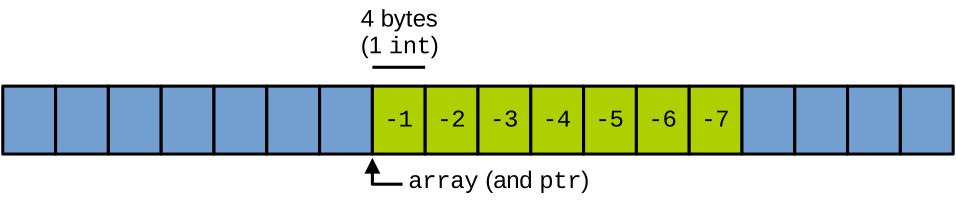
As you can see, the array array and the pointer ptr are equivalent: they both represent a pointer to the first byte of the array in memory:
Custom Data Structures and Pointers
In C, we very often create pointers to custom data structures.
Here we have an example with ptr pointing to ms.
typedef struct {
    int x;
    float f;
    char *s;
} my_struct;

my_struct ms = {42, 2.5, "hello"};
my_struct *ptr = &ms;

printf("%d\n", (*ptr).x); // prints "42"
To access a field of ms, we need to dereference the pointer first with the * operator, then access the field with the . operator.
Parentheses are needed here because of operator precedence.
Writing all this is a bit cumbersome, so as a shortcut you can use the arrow operator ->, which both dereferences the pointer on its left and accesses the field on its right:
printf("%s\n", ptr->s); // prints "hello", equivalent to (*ptr).s
Pointers Chains
Because a pointer is a variable, it can itself be pointed to by another pointer. We talk in that case of a pointer of pointer. And with this we can create pointer chains linking memory locations. Consider the following code:
int value = 42;         // integer
int *ptr1 = &value;     // pointer of integer
int **ptr2 = &ptr1;     // pointer of pointer of integer
int ***ptr3 = &ptr2;    // pointer of pointer of pointer of integer

printf("ptr1: %p, *ptr1: %d\n", ptr1, *ptr1);
printf("ptr2: %p, *ptr2: %p, **ptr2: %d\n", ptr2, *ptr2, **ptr2);
printf("ptr3: %p, *ptr3: %p, **ptr3: %p, ***ptr3: %d\n",
        ptr3, *ptr3, **ptr3, ***ptr3);
We have an integer value.
ptr1 is a pointer of int, i.e., an int *, and points to the integer.
Then we want to have something that points to ptr1: that’s a pointer of pointer of int, an int **.
It’s ptr2, whose value is the address of ptr1.
Then we create another level in the chain with ptr3, which is a pointer of pointer of pointer of int, an int ***, pointing to ptr2.
And next we print the value of each pointer in the chain and what they point to.
The chain can be illustrated as follows:

Function Pointers
Function pointers are a special type of pointer that reference functions.
Rather than taking the address of some data, they take the address of machine code.
More precisely, a function pointer pointing to function f takes as value the address of the first byte of machine code of the function f.
Consider the following example:
#include <stdio.h>

void greet_v1(char *name) {
  printf("Good morning, %s!\n", name);
}

void greet_v2(char *name) {
  printf("Good evening, %s!\n", name);
}

int main() {
  // declare a function pointer to a function that returns void
  // and takes a char * as parameter:
  void (*func_ptr)(char *);
  char *username = "Pierre";

  func_ptr = greet_v1;  // set func_ptr to point to greet_v1
  func_ptr(username);   // call greet_v1 through the pointer

  func_ptr = greet_v2;  // set func_ptr to point to greet_v2
  func_ptr(username);   // call greet_v2 through the pointer

  return 0;
}
A function pointer is declared with the return type of the pointed function (here void), the name of the pointer (here func_ptr), and the type or types of parameters of the pointed function, here a single parameter char *.
A function pointer can then be set to point to various functions fitting the prototype it was defined with; here we make it point to greet_v1 and then greet_v2.
This is a simple assignment using the function name to obtain its address.
The function pointer can be called by using its name as one would do for a function.
C: Dynamic Memory Allocation
You can access the slides 🖼️ for this lecture.
Here we cover dynamic memory allocation, which corresponds to manual allocation of memory by the programmer. This is extensively used in C to allocate memory for large quantities of data or for data structures whose size is not known at compile time (e.g., user input).
Motivation
So far we looked at programs in which the total amount of memory needed for their data and code was known at compile time. As a result, the compiler handles all memory allocation automatically. This is called static memory allocation. However, there are situations where we need to reserve some memory whose size is not known until runtime.
Consider the following program:
void process_array(int size) {
    int arr[size];  // variable-size array,
                    // not a great solution
    for (int i = 0; i < size; i++){
        arr[i] = i * i;
        printf("%d\n", arr[i]);
    }
}

int main() {
    int n;
    printf("Enter the size of the array: ");
    scanf("%d", &n);
    if (n > 0) process_array(n);

    printf("all good\n");
    return 0;
}
This code asks the user for a number with the scanf function.
That number is then passed to a function that allocates an array whose size is based on that number.
The size will only be known at runtime because it depends on the number entered by the user.
What we have here is a variable-sized array, which is generally a bad practice in C.
As a local variable, arr is stored in an area of the address space called the stack.
The stack has a very small size, just a few megabytes on modern general-purpose OSes such as Linux.
As a result, if the user enters a number that is too large, the stack will overflow and the program will crash or misbehave.
If you try it out and input 100000000000000, the program will crash and be terminated by the OS as follows:
$ gcc variable-size-array.c -o prog
$ ./prog
Enter the size of the array: 100000000000000
[1]    17467 segmentation fault (core dumped)  ./prog
We need a better solution.
malloc and free
The programmer manually allocates memory with a function called malloc, and when that memory is no longer needed by the program it must be released manually with a function called free.
malloc.
To allocate at runtime memory whose size is 1) unknown at compile-time and/or 2) potentially large, in C we must use the malloc function.
Its prototype is as follows:
void *malloc(size_t size);
malloc accepts a single parameter, size, which specifies the amount of bytes to allocate.
It allocates a contiguous area of memory in the address space (we call that a buffer), and returns a pointer to the first byte of that area, or NULL if the allocation failed.
One important point to note is that, although for allocation requests of reasonable sizes malloc will almost always succeed, in practice we can never be certain of the outcome of the allocation.
Indeed, the system may be running low on memory and unable to satisfy certain calls to malloc.
As a result, it is important to always check that the return value of malloc is not NULL before starting to use the allocated memory.
If malloc returns NULL, you also need to take appropriate action, for example exit the program with an error message.
Also note that malloc returns a void * pointer: it is a generic pointer that can be transformed into a pointer to any other type through an operation called a cast.
As a result, malloc can allocate memory that can hold any type of data.
free.
Any area of memory allocated manually by the programmer with malloc must also be released manually when it is no longer needed.
This is done with the free function, whose prototype is:
void free(void *p);
free takes the pointer returned by malloc as a parameter, i.e., the first byte of the memory area to release.
We can now see malloc and free in action in the following example.
This is an adaptation of our previous program that was using variable-sized arrays, this time using dynamic memory allocation:
void process_array(int size) {
  // Allocate an area of memory large enough to contain n integers:
  int *arr = (int *)malloc(size * sizeof(int));

  if(arr == NULL) { // ALWAYS check malloc's return value, if it fails we just exit
    printf("ERROR: cannot allocate memory\n");
    exit(-1);
  }

  for (int i = 0; i < size; i++)
        arr[i] = i * i;

  free(arr); // release memory with free
}
You can observe that the function allocating the array starts by calling malloc.
It requests enough space to store size integers, so the parameter passed to malloc is size * sizeof(int).
The (int *) before malloc is our cast: we transform the void pointer it returns into an int pointer, which, as you recall from the previous video, points to an array of integers.
We then need to check that the allocation succeeds.
If it fails, we print an error message and exit.
If successful, we can iterate over the array normally and populate it.
Once we are done, we can release the memory using free.
Memory Leaks
It is important not to forget to release memory allocated with malloc when it is no longer needed.
A program that fails to release memory it has allocated with malloc is said to have a memory leak.
Leaks are a security issue: they can be exploited by an attacker to crash the program or starve the machine of resources.
The code below is a buggy program, an adaptation of our previous example in which the free call was removed:
void process_array(int size) {
  // Allocate an area of memory large enough to contain n integers:
  int *arr = (int *)malloc(size * sizeof(int));

  if(arr == NULL) { // ALWAYS check malloc's return value, if it fails we just exit
    printf("ERROR: cannot allocate memory\n");
    exit(-1);
  }

  for (int i = 0; i < size; i++)
        arr[i] = i * i;

  // No free! At that stage the pointer arr is gone so the memory will never be freed!
  // It's a leak of size * sizeof(int) bytes
}
This program is incorrect and allocates memory that is never freed: it leaks memory.
On Linux, a command-line tool named Valgrind can help identify leaks, among other memory errors.
To help understand the output of Valgrind, it is useful to embed debug symbols into the program’s binary at compile time with the -g switch:
$ gcc -g my-leaky-program.c -o my-leaky-program
We can then run the program under Valgrind:
$ valgrind --leak-check=full  ./my-leaky-program   # invoke valgrind
# ...
Enter the size of the array: 100
==144325==
==144325== HEAP SUMMARY:
==144325==     in use at exit: 400 bytes in 1 blocks
==144325==   total heap usage: 3 allocs, 2 frees, 2,448 bytes allocated
==144325==
==144325== 400 bytes in 1 blocks are definitely lost in loss record 1 of 1
==144325==    at 0x48407B4: malloc (vg_replace_malloc.c:381)
==144325==    by 0x109194: process_array (my-leaky-program.c:5)
==144325==    by 0x109235: main (my-leaky-program.c:25)
==144325==
==144325== LEAK SUMMARY:
==144325==    definitely lost: 400 bytes in 1 blocks
==144325==    indirectly lost: 0 bytes in 0 blocks
==144325==      possibly lost: 0 bytes in 0 blocks
==144325==    still reachable: 0 bytes in 0 blocks
==144325==         suppressed: 0 bytes in 0 blocks
Valgrind reports that 400 bytes of memory have been leaked, and provides some information about where the leak comes from, so it can be fixed. Please make sure to use Valgrind to check for leaks in all the C code you produce as part of this unit. Leaks are a bug and a security issue, and your code should be free from them.
The C Standard Library
You can access the slides 🖼️ for this lecture.
Here we discuss the C standard library, a collection of functions to accomplish various tasks when writing C programs.
Introduction
The C standard library, also shortened as libc, provides a set of pre-written functions to accomplish a plethora of low-level tasks in C.
We have seen a few of these functions already: printf to print to the console, malloc to allocate memory, and a few others.
These functions are portable, and you can use them with any compiler, operating system, and target architecture.
The libc functions fall within a series of broad categories:
- Input/output (
stdio.h) - Memory management (
stdlib.h) - String and memory manipulation (
string.h) - Mathematical functions (
math.h) - File handling (
fcntl.h,unistd.h) - Time and date (
time.h)
To use the functions from the libc, the programmer needs to include the relevant header .h files.
Here we focus on some memory/string manipulation functions, because they have security implications.
String Copy
char *strcpy(char *dest, const char *src);
char *strncpy(char *dest, const char *src, size_t n);
The function strcpy lets the programmer perform a string copy.
It takes as parameters the destination buffer and the source string.
The destination should be a buffer with enough space to accommodate a copy of the source.
A variant is strncpy, which takes another parameter, n.
strncpy will do the copy up to a maximum of n characters.
You can see an example of the usage of both functions below:
#include <string.h>
/* ... */
char *string1 = "hello";
char *string2 = string1;   // this is not a string copy!
char string3[10];          // allocated space of 10 bytes, it's called a buffer

/* not super safe, what happens if the size of string1 is larger than the
 * 10 bytes available in string3? */
strcpy(string3, string1);

/* better */
strncpy(string3, string1, 10);

printf("string1 @%p: %s\n", string1, string1); // string1 @1234: hello
printf("string2 @%p: %s\n", string2, string2); // string2 @1234: hello
printf("string3 @%p: %s\n", string3, string3); // string3 @5678: hello
We have a string named string1, containing "hello".
Look at how string2 is constructed: please note that this is not a string copy: the assignment simply places the value of string1, which is a pointer, into string2.
We end up with another pointer pointing to the original string:

If you want to make a proper string copy, i.e. to copy all characters from one memory location to another, you need to use strcpy.
This is what happens to string3: it points to a buffer of 10 characters which is enough to accommodate a copy of the original string.
Then we call strcpy, which will in effect copy the source into the destination, including the termination character.
Note that strcpy can be dangerous when the source string is larger than the destination buffer: the function will blindly copy the entire source string and will overflow the destination buffer.
To help avoid this, you can use strncpy, and pass as its last parameter the size of the destination buffer.
String Concatenation
char *strcat(char *dest, const char *src);
char *strncat(char *dest, const char *src, size_t n);
To concatenate one string to another, you can use strcat.
It takes two strings as parameters, a destination and a source.
After the call, the destination string will contain the concatenation of the original destination string, followed by the source string.
Once again, make sure the destination buffer has enough space to accommodate the sum of characters of the original destination, the source, plus one termination character.
If you want to concatenate up to a certain number of characters, you can use strncat.
Below is an example of the usage of these functions:
#include <string.h>

/* ... */

char world[6] = "world";
char s1[32];
char s2[32];

strcpy(s1, "hello ");
strcpy(s2, "hello ");

strcat(s1, world);       // not very safe
strncat(s2, world, 32 - strlen(s2));  // better

printf("s1: %s\n", s1); // hello world
printf("s2: %s\n", s2); // hello world
We have 2 buffers of 32 bytes each, s1 and s2.
We start by placing the string "hello " in each buffer with strcpy.
Then we concatenate s1 and the "world" string, resulting in s1 being "hello world".
We also have a safer example with strncat concatenating s2 and the "world" string.
See how we calculate the maximum number of characters to concatenate: it is the size of the destination buffer (32 bytes) minus the number of characters already present in it, obtained with the strlen function that returns the length of a string.
Copying Memory
void *memcpy(void *dest, void *src, size_t n);
To copy memory from one place to another we can use the memcpy function.
It’s better to use that function than to copy manually, because it is highly optimised for speed.
memcpy copies n bytes from the source src into the destination dest.
Note that the source and destination are void * generic pointers so they can point to anything.
Here is an example of the usage of memcpy:
# include <string.h>

typedef struct {
    int m1; int m2; int m3; float f1;
} mystruct;

int main() {
  int array_size = 10;
  mystruct array1[array_size];
  mystruct array2[array_size];

  for(int i=0; i<array_size; i++) { // initialise all of array1's members
    array1[i].m1 = /* ... */;
    array1[i].m2 = /* ... */;
    array1[i].m3 = /* ... */;
    array1[i].f1 = /* ... */;
  }

  // Assume we want to make a copy of array1 into array2: using memcpy is easier
  // (and faster) than using a loop:
  memcpy(array2, array1, array_size*sizeof(mystruct));
}
We have 2 arrays of 10 elements, each element being a relatively large data structure.
We populate the first array manually, then suppose we want to populate the second array with the same content.
Because we know that 1-dimensional arrays are laid out contiguously in memory, we can achieve this quickly with a memcpy.
So we call memcpy with the destination being array2 and the source being array1.
Remember that in C, arrays are pointers so we can pass them as parameters to memcpy.
We also calculate the number of bytes to copy: it is the number of elements in the arrays, multiplied by the size of each element obtained with sizeof.
Console Input
char *fgets(char *s, int size, FILE *stream);
int scanf(const char *format, ...);
To get a string of characters from the user, you can use fgets.
It takes the destination buffer s as a parameter, as well as the maximum number of characters to write, size.
The third parameter is a stream that we’ll use to indicate that the characters should come from the console, also called the standard input.
To get numbers from the user, you can use scanf.
It takes a string describing the input format as its first parameter, followed by the addresses of the variables to fill with the input.
The code below illustrates the use of fgets and scanf:
int int1, int2;
double double1;
float float1;
char s[128];

printf("Please input a string:\n");
fgets(s, 128, stdin);

printf("Please input an integer:\n");
scanf("%d", &int1);

printf("Please input a float:\n");
scanf("%lf", &double1); /* make sure to use %lf for double and %f for float */

printf("Please enter an integer and a float separated by a space\n");
scanf("%d %f", &int2, &float1);

printf("You have entered: %d, %d, %lf, %f, and %s\n",
        int1, int2, double1, float1, s);
The first call to fgets here gets a string from the user and places it into a buffer of 128 characters.
Then we have a few calls to scanf to get respectively an integer, a double, and, on a single line, an integer and a float separated by a space.
The program then prints the values of each number and string input to the program.
More Libc Functions, Manual Pages
Obviously, we cannot make a comprehensive overview of all functions from the C standard library here. In the rest of the unit, there will be other functions that will be useful to you, either because we are seeing them in the lecture materials, or because you need to use them to complete the lab exercises. To search and explore what kind of functions are available, there are many solutions, but one good starting point is cppreference.com, which has a good section on the C language and its standard library.
Furthermore, if you want to know how to use a particular function of the libc, you can use the manual.
In a Linux terminal, run the man command followed by the name of the function:
man <function name>
The man page of the function in question will be displayed, describing the function’s prototype, its behaviour, the headers you need to include to use the function, and the values it can return on success or on failure. To exit the man page, simply type q on your keyboard.
⚠️ If a libc function name clashes with a command line program name, you may need to look up a different section of the manual. An example here is the
syncfunction, which flushes filesystem RAM caches to disk.sync()is a function of the libc, butsyncis also a terminal program.man syncwill show the man page for the terminal program, so to check the page for the libc function, look up section 2 of the manual:man 2 sync
C: Further Readings
General Security Concepts
- Saltzer and Schroeder, The Protection of Information in Computer Systems. A classic, seminal paper on the topic of computer systems security.
- Lampson, Protection. Another seminal paper in systems security.
- Thomas, Selected Systems Engineering Process Deficiencies and Their Consequences. Describes a few aeronautics and space systems engineering failures, including the case of Ariane 5.
- Wilson and Jayawardena, Dirty Cow Demo. A visual explanation of Linux’s Dirty Cow vulnerability.
- Lipp et al., Meltdown: Reading Kernel Memory from User Space, and Kocher et al., Spectre Attacks: Exploiting Speculative Execution. Two papers describing the Meltdown and Spectre hardware CPU side channels.
- Zanero, Coming of Age - Stressing the Importance of Threat Models. “The only way to reason sensibly about the security of a system, the closest thing we have to a method in the madness of this field, is to start from a realistic and complete model of the threats and the attack surface of the system.”
C Programming Language
- The lecture notes for my BSc. course unit on C. A much more detailed overview of the language.
- cppreference.com, C. Good reference for the language.
- learn-c.org. Exercises you can do in your browser.
- Harvard’s CS50. The materials from week 1 to 4 cover C.
Anatomy of a Program in Memory
You can access the slides 🖼️ for this lecture.
Before analysing the types of attacks that arise from software vulnerabilities and the defences designed to mitigate them, it is essential to understand how programs behave at runtime. Attackers who target low-level system software try to trigger bugs in the program. They then use their deep understanding of how the software behaves to turn such bug-induced malfunctions into real attacks. Hence, on the defence side, if we want to build secure programs and protect software, we need a good understanding of what happens on the CPU and in memory when a program runs.
The Virtual Address Space
Each program sees the memory it can access as a very large array of bytes, the address space. Each slot in this array has an address, from 0 to ~256 TB on modern 64-bit CPUs. The program accesses memory with load and store instructions at target addresses. On Linux the OS kernel is mapped in the address space of each running program, and reserves the upper half of that address space for itself. That leaves the lower 128 TB for the program: it is free to perform load and store operations anywhere in that area.

Virtual Memory. Virtual memory allows creating such a very large address space independently of the amount of RAM that the computer is equipped with. Each program running on the system also gets its own, private address space, and is free to perform loads/stores anywhere in the lower half of that address space without disturbances from other programs: without establishing any form of communication, programs do not see each other’s address spaces.
To achieve these goals, virtual memory performs address translation: after virtual memory is enabled very early in the boot process, any address used by the CPU to index a load/store operation will be a virtual address. Virtual addresses are mapped by the memory management unit (MMU) to physical addresses that index the actual RAM of the computer. This mapping is realised on modern processors with a data structure called the page table:
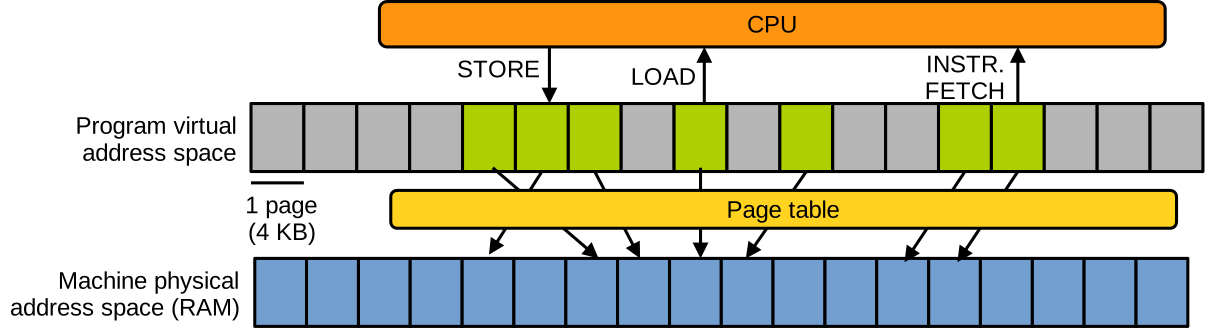
The mapping is realised at the granularity of a page (4 KB). Each program running on the system gets its own page table defining a different mapping, making sure no physical page is mapped into the address spaces of two different programs. The page table also allows the virtual address space to be sparsely populated: most virtual pages are not mapped to physical memory.
Virtual Address Space Life Cycle
How does the address space evolve during the execution of a program? Part of it is set up at load time, when the program is invoked, and before it starts executing. Part of the address space also evolves and changes at runtime.
When a program is invoked (e.g., the user types ./inspect-me on the command line), the operating system first creates a virtual address space for the program’s execution.
Before the program can run, its binary must be loaded inside that address space.
The program’s binary lives somewhere on the computer’s disk.
The binary is in a particular format (for Linux it is ELF, which stands for Executable and Linkable Format).
The format’s metadata embedded in the binary indicate what tool should be used to bootstrap the address space: this is called the loader.
The loader is a separate binary from the program we want to execute, and on modern Linux distributions it is generally named after a variant of ld-linux.so.
Once the loader is identified, the OS loads the loader by mapping parts of its binary (loader code and data) in the address space:
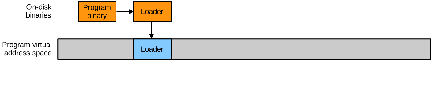
We can inspect the ELF metadata for a particular program binary with the readelf tool.
For example, to see information about the loader required to run the program ls:
$ readelf -l /bin/ls
...
      [Requesting program interpreter: /lib64/ld-linux-x86-64.so.2]
...
Once the loader is loaded, it starts to execute, reads more ELF metadata from the program’s binary, and with that information it can load the program’s binary into the address space:
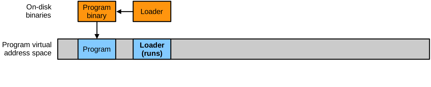
Most programs are dynamically linked: loading their binary alone is not sufficient to prepare their execution, and they require additional libraries to be loaded.
Most libraries today, on operating systems like Linux or Windows, are called shared libraries, as they can be loaded into the address spaces of several programs.
The C standard library is itself available by default as a shared library (libc.so).
The loader fetches the list of libraries required for the program’s execution from the ELF metadata of the program’s binary.
$ ldd /bin/ls
	linux-vdso.so.1 (0x00007f847f8eb000)
	libcap.so.2 => /usr/lib/libcap.so.2 (0x00007f847f871000)
	libc.so.6 => /usr/lib/libc.so.6 (0x00007f847f600000)
	/lib64/ld-linux-x86-64.so.2 => /usr/lib64/ld-linux-x86-64.so.2 (0x00007f847f8ed000)
We can see that ls requires a few shared libraries, including the C standard library and the loader.
When the shared library dependencies are identified, the loader loads the corresponding binaries into the address space:
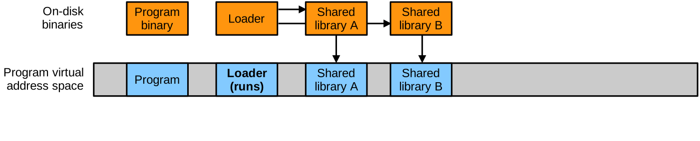
Static Memory. At that stage the program is ready to run, and all the memory set up in the address space is called static memory. The term static comes from the fact that the sizes of these areas (space reserved for the data/code they contain) are fixed at compile time, and will not change throughout the program’s entire execution. Static memory mostly includes executable code and global variables. When static memory is set up, the program can start to execute.
Dynamic Memory. As it runs, the program will also need dynamic memory, i.e. areas whose sizes are not known at compile time and will evolve at runtime. The program needs a stack that will handle function calls and returns. The stack is a contiguous area of memory used to hold function arguments, local variables, function return values and return locations in the code. With each function call, the stack grows, and it shrinks when a function returns. On most architectures the stack grows down, i.e. from high to low addresses.
A second important area of dynamic memory is the heap.
This is where memory allocated dynamically with malloc lives.
The way the heap grows/shrinks can differ depending on the implementation: it either grows upwards towards higher addresses, or it can correspond to an area that is not necessarily contiguous and spread over the address space.
Dynamic memory also includes other mappings made at runtime in the virtual address space: these can be file mappings (e.g., dynamically loaded modules), executable areas for just-in-time compiled code, etc. Static and dynamic memory areas can be illustrated in our example as follows:
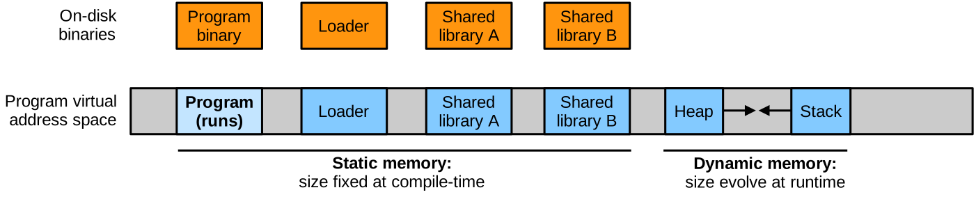
All the areas of the virtual address space have access permissions. These permissions are set up by the OS and enforced by the CPU on each load and store operation. Code areas are generally set to be executable and possibly readable, while data areas are set to be readable and writable or possibly read-only, etc.
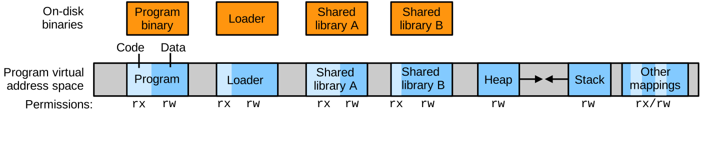
Memory Map of a Process
On Linux, the /proc pseudo-filesystem provides a convenient way to inspect operating system-level information about running programs, including their memory maps.
An executing program’s memory map lists the areas of the program’s virtual address space that are mapped to physical memory, their location, permissions, etc.
To inspect a program’s memory map, simply display the file /proc/<program's PID>/maps:
$ cat /proc/21184/maps
564870330000-564870331000 r--p 00000000 103:04 35652325  /home/pierre/prog
564870331000-564870332000 r-xp 00001000 103:04 35652325  /home/pierre/prog
564870332000-564870333000 r--p 00002000 103:04 35652325  /home/pierre/prog
564870333000-564870334000 r--p 00002000 103:04 35652325  /home/pierre/prog
564870334000-564870335000 rw-p 00003000 103:04 35652325  /home/pierre/prog
56489d9a4000-56489d9c5000 rw-p 00000000 00:00 0          [heap]
7f6b9ec32000-7f6b9ec35000 rw-p 00000000 00:00 0
7f6b9ec35000-7f6b9ec5b000 r--p 00000000 103:04 27004964  /usr/lib/x86_64-linux-gnu/libc.so.6
7f6b9ec5b000-7f6b9edb0000 r-xp 00026000 103:04 27004964  /usr/lib/x86_64-linux-gnu/libc.so.6
7f6b9edb0000-7f6b9ee03000 r--p 0017b000 103:04 27004964  /usr/lib/x86_64-linux-gnu/libc.so.6
7f6b9ee03000-7f6b9ee07000 r--p 001ce000 103:04 27004964  /usr/lib/x86_64-linux-gnu/libc.so.6
7f6b9ee07000-7f6b9ee09000 rw-p 001d2000 103:04 27004964  /usr/lib/x86_64-linux-gnu/libc.so.6
7f6b9ee09000-7f6b9ee16000 rw-p 00000000 00:00 0
7f6b9ee2e000-7f6b9ee30000 rw-p 00000000 00:00 0
7f6b9ee30000-7f6b9ee31000 r--p 00000000 103:04 27004961  /usr/.../ld-linux-x86-64.so.2
7f6b9ee31000-7f6b9ee56000 r-xp 00001000 103:04 27004961  /usr/.../ld-linux-x86-64.so.2
7f6b9ee56000-7f6b9ee60000 r--p 00026000 103:04 27004961  /usr/.../ld-linux-x86-64.so.2
7f6b9ee60000-7f6b9ee62000 r--p 00030000 103:04 27004961  /usr/.../ld-linux-x86-64.so.2
7f6b9ee62000-7f6b9ee64000 rw-p 00032000 103:04 27004961  /usr/.../ld-linux-x86-64.so.2
7ffd9db2f000-7ffd9db50000 rw-p 00000000 00:00 0          [stack]
7ffd9dba3000-7ffd9dba7000 r--p 00000000 00:00 0          [vvar]
7ffd9dba7000-7ffd9dba9000 r-xp 00000000 00:00 0          [vdso]
Each entry includes the start and end addresses of the corresponding area in the virtual address space.
Many entries are file mappings, and correspond to binaries being loaded in the address space.
We can identify the running program’s binary (prog), the C standard library (libc.so.6) and the loader (ld-linux-x86-64.so.2).
These all correspond to static memory.
Regarding dynamic memory, we can identify the stack and the heap.
Each area has a set of access permissions such as read (r), write (w), and execute (x).
Regions marked r-x typically correspond to executable code regions of the program or shared libraries.
Writable and read-only regions hold data.
Loading Process, Static Memory
If we zoom in on the loading process for an ELF binary (main program, loader, or shared libraries), the on-disk binary file’s content is divided into sections. When the binary is loaded, contiguous sections with similar permissions form segments that are mapped in the address space:
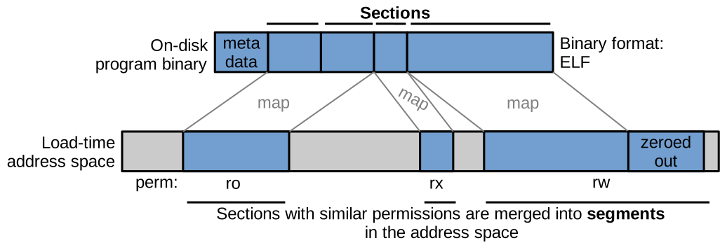
This mapping corresponds in essence to copying the content of the section into memory at the relevant location in the address space, and setting up the proper permissions: this is generally realised with the mmap system call.
Private mappings are used for the ELF binaries, meaning that stores by the program in writable areas will not be reflected in the binaries on disk.
After load time, other mappings will be created at runtime, for example to hold the heap and the stack.
These are anonymous mappings, meaning they are not backed by any file.
We can inspect an ELF binary with readelf to see the sections it contains and the segments that will be created in the address space at runtime:
$ readelf -lSW inspect-me
There are 31 section headers, starting at offset 0x36f8:

Section Headers:
  [Nr] Name              Type            Address          Off    Size   ES Flg Lk Inf Al
  [15] .text             PROGBITS        0000000000001070 001070 00011f 00  AX  0   0 16
  [17] .rodata           PROGBITS        0000000000002000 002000 000008 00   A  0   0  4
  [25] .data             PROGBITS        0000000000004018 003018 000010 00  WA  0   0  8
  [26] .bss              NOBITS          0000000000004028 003028 000008 00  WA  0   0  1

...

Program Headers:
  Type           Offset   VirtAddr           PhysAddr           FileSiz  MemSiz   Flg Align
  LOAD           0x000000 0x0000000000000000 0x0000000000000000 0x000688 0x000688 R   0x1000
  LOAD           0x001000 0x0000000000001000 0x0000000000001000 0x000199 0x000199 R E 0x1000
  LOAD           0x002000 0x0000000000002000 0x0000000000002000 0x0000e0 0x0000e0 R   0x1000
  LOAD           0x002dd0 0x0000000000003dd0 0x0000000000003dd0 0x000258 0x000260 RW  0x1000

...

 Section to Segment mapping:
  Segment Sections...
   03     .init .plt .plt.got .text .fini
   04     .rodata .eh_frame_hdr .eh_frame
   05     .init_array .fini_array .dynamic .got .got.plt .data .bss
readelf prints for each section its offset (Off, location of the start of the section on disk), its size, permissions (Flg, with X for executable and W for writable), and other information such as alignment constraints.
Similar information is available for segments, with their location and size in the address space (VirtAddr and MemSiz), along with permissions and alignment information.
Finally, readelf also outputs the list of sections composing each segment: you can confirm that it is always sections with similar permissions that are merged together into a segment.
The Code Segment
The code segment for a loaded binary contains the machine code to be executed by the CPU for the corresponding program/library.
It is possible to see the content of the code segment for a binary by disassembling it.
We can illustrate that with an example.
Consider this C program, inspect-me.c:
#include <stdio.h>
#include <unistd.h>

int main(int argc, char **argv) {
    while(1) {
        printf("%d\n", getpid());
        sleep(1);
    }
    return 0;
}
We can compile inspect-me.c into the ELF binary inspect-me and disassemble it:
$ gcc inspect-me.c -o inspect-me
$ objdump --disassemble inspect-me

...

0000000000001159 <main>:
    1159: push   %rbp
    115a: mov    %rsp,%rbp
    115d: sub    $0x10,%rsp
    1161: mov    %edi,-0x4(%rbp)
    1164: mov    %rsi,-0x10(%rbp)
    1168: call   1030 <getpid@plt>
    116d: mov    %eax,%esi
    116f: lea    0xe8e(%rip),%rax
    1176: mov    %rax,%rdi
    1179: mov    $0x0,%eax
    117e: call   1040 <printf@plt>
    1183: mov    $0x1,%edi
    1188: call   1050 <sleep@plt>
    118d: jmp    1168 <main+0xf>
What we see here are the x86-64 machine instructions making up the code for the main function.
The hexadecimal number before each instruction is the offset at which that instruction is located in the binary’s code section.
Function Calling Convention
While we are looking at machine code, an important thing to know in order to understand this week’s content is: which assembly instructions are executed upon function calls and returns. The concept of a “function” does not really exist at the machine code level: if you disassemble a program compiled from a source file having multiple functions, you will see that all the functions’ code is merged into the code segment.
At compile time, the compiler generates the machine code for function calls and returns according to an architecture-specific calling convention. For x86-64, the convention used for Linux is the System V x86-64 Application Binary Interface (ABI). The convention states that the machine code implementing function calls and returns should follow these rules:
- Upon a function call, the calling function (caller) first places its arguments, in order, in the registers
%rdi,%rsi,%rdx,%rcx,%r8, and%r9(these are x86-64 general-purpose registers). It then issues thecallinstruction, which makes the CPU jump to the first instruction of the called function (callee) in the code segment.- If the callee has more than 6 parameters, additional parameters are pushed on the stack.
- When a function returns, the callee places the return value in the
%raxregister and executes theretinstruction: the CPU jumps back to the next instruction following thecallin the caller.
Anatomy of a Function Call.
If we study the machine code obtained by disassembling inspect-me above and look at the invocation of the getpid and printf functions within main, we have the following assembly instructions:
1168: call   1030 <getpid@plt>
116d: mov    %eax,%esi
116f: lea    0xe8e(%rip),%rax
1176: mov    %rax,%rdi
...
117e: call   1040 <printf@plt>
We can see the following happening:
1168:getpidtakes no argument, so it can be called directly with acallinstruction116d: the return value ofgetpidis in%rax; it is moved into%esi(%eaxand%esiare the lower 32 bits of the 64-bit registers%raxand%rsi): this is the preparation of the second argument for the upcoming call toprintf116fand1176: the address of the string"%d\n"is loaded into%rax(it is computed as the offset0xe8efrom the current instruction pointer), then moved into%rdi: this is the preparation of the first argument for the upcoming call toprintf117e:printfis called with acallinstruction
Anatomy of a Function Return. An important concept for this week’s content is: how does the CPU know where to jump back to when returning from a function call? Similar to what we saw with a function call, let’s study what happens at the machine code level when a function returns. Consider the following code:
int f(int param) {
  int f_local = 0xcafe;
  /* ... */
  return 0x33;
}

int main() {
  int main_local = 0x42;
  int ret = f(main_local);
  /* ... */
}
Compiled and disassembled, we see the following:
0000000000001139 <f>:
  1139:	55                   	push   %rbp
  113a:	48 89 e5             	mov    %rsp,%rbp
  113d:	89 7d ec             	mov    %edi,-0x14(%rbp)
  1140:	c7 45 fc fe ca 00 00 	movl   $0xcafe,-0x4(%rbp)
  1147:	b8 33 00 00 00       	mov    $0x33,%eax ; 6. return value placed in %rax
  114c:	5d                   	pop    %rbp       ; 7. return from f into main
  114d:	c3                   	ret

000000000000114e <main>:
  114e:	55                   	push   %rbp
  114f:	48 89 e5             	mov    %rsp,%rbp
  1152:	48 83 ec 10          	sub    $0x10,%rsp
  1156:	c7 45 f8 42 00 00 00 	movl   $0x42,-0x8(%rbp)  ; 1. main_local = 0x42;
  115d:	8b 45 f8             	mov    -0x8(%rbp),%eax   ; 2. 0x42 loaded in %rax
  1160:	89 c7                	mov    %eax,%edi         ; 3. 0x42 moved to %rdi
  1162:	e8 d2 ff ff ff       	call   1139 <f>          ; 4. call f
  1167:	89 45 fc             	mov    %eax,-0x4(%rbp)   ; 5. store return value in ret
  116a:	b8 00 00 00 00       	mov    $0x0,%eax
  116f:	c9                   	leave
  1170:	c3                   	ret                      ; 8. return from main
We can see that the System V convention we described earlier is well followed: before calling f, main prepares its argument by placing 0x42 into %edi.
f is called with a call instruction.
Inside f, when it is time to return to main, the return value 0x33 is placed into %rax, and the return is made with a ret instruction.
When f returns, main places the return value in a local variable and then returns itself with a ret instruction.
Compare the invocation of the call and ret instructions and consider where does the CPU need to jump?
For calls, it is easy: there is always a single target address in the code segment, as we always call a particular function; for example, when main calls f, the CPU jumps to offset 0x1139.
For ret things are a bit more complicated because a function can be called from many different locations in a program, so there is no single return point and the compiler can’t embed a single return address in the code like it does with call.
The return address is actually pushed on the stack upon each function call.
Function Calls and the Stack
We have seen that the stack is a contiguous area in the address space that holds per-function data, e.g., parameters and local variables.
Each function has a stack frame on the stack: an area of contiguous memory dedicated to holding information and data for that particular function.
With our example, when main runs, before it calls f the stack looks like this:
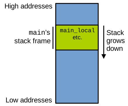
When main calls f, it executes the call instruction.
As a result the CPU:
- Pushes the return address (the location in
mainwhere execution should resume) on the stack; and - Jumps to the target function
f.
Then f starts to run and allocates a frame for itself on the stack.
At that stage, the stack looks as follows: main’s frame, followed by the return address for the call to f, followed by f’s frame:
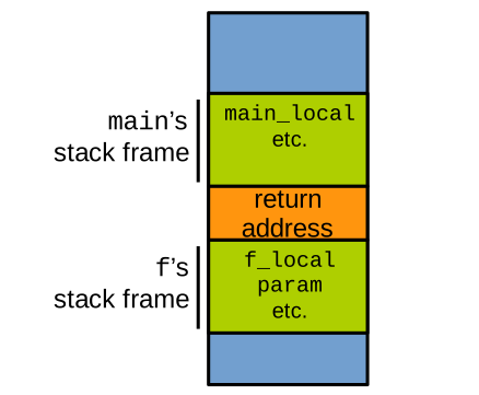
When f is done, it discards its stack frame and returns to main by executing the ret instruction.
As a result the CPU:
- Pops the return address from the stack; and
- Jumps to it.
main can continue to execute, starting at the next instruction after the call.
This way, even if functions can be called from multiple locations in the program, including in a nested manner, the CPU always knows the proper location in the code where to jump back when a function returns.
Memory Safety
You can access the slides 🖼️ for this lecture.
The concept of memory safety relates to making sure that the CPU running a program accesses memory at the right location and at the right moment. This is enforced in memory-safe languages such as Python or Java with a series of checks and mechanisms that, for various reasons, are unfortunately absent in the most popular languages used to write systems software, C and C++: they are memory-unsafe. This has severe security implications. Here we present the concept of memory safety in detail.
Introduction
Memory safety is about protecting a program from a whole class of bugs that arise when the program accesses memory it should not, for example, when indexing an array out of bounds, overflowing a buffer, or accessing freed memory. Some of the protections against these issues are applied at compile time, and others at runtime. A major problem is that the programming languages used to write most systems software, C and C++, lack most of these protections: we say that C and C++ are not memory safe. When memory safety violations occur, not only can the program crash or exhibit strange behaviour, but, more concerning, these violations represent security issues that can be exploited by attackers to compromise availability (for example, crash a program or a system), confidentiality (leak sensitive data/secrets), and integrity (corrupt important data or code, for example, to escalate privileges).
Memory Safe vs. Unsafe Languages
Memory Safe Languages.
Contrary to C and C++, high-level languages such as Java or Python are said to be memory safe.
They enforce a series of rules at compile time and/or runtime to prevent memory safety violations.
These rules include checking for out-of-bounds accesses, preventing deallocated memory from being accessed or even referenced, making sure that memory can be deallocated only once, and that invalid references such as NULL pointers cannot be dereferenced, making sure that memory is always initialised before being read, and is always accessed through variables of the proper type, etc.
Here is an example of buggy code in Python, where we access an array out of bounds:
numbers = [1, 2, 3]
# Python will throw an out-of-bounds exception here:
print("The fourth number is:", numbers[3])
If you try that code, you’ll get an exception: Python performs a bounds check at runtime when the array is indexed:
$ python3 out-of-bounds.py
Traceback (most recent call last):
  File "/tmp/out-of-bounds.py", line 3, in <module>
    print("The fourth number is:", numbers[3])
                                   ~~~~~~~^^^
IndexError: list index out of range
Memory Unsafe Languages. As we mentioned, contrary to higher-level languages, the most popular languages for systems software, C and C++, are not memory safe. They lack the majority of the memory safety violation checks we mentioned:
- There are no checks for out-of-bounds array and buffer accesses;
- There are no checks for the presence of pointers to deallocated memory or their dereferencing;
- There are no checks for buggy behaviour such as double frees on the same buffer, the dereferencing of invalid or
NULLpointers, or reading uninitialised memory; - The type checking system of C/C++ can easily be bypassed, for example, with casts (which are often needed to write functional programs).
Here is an equivalent C implementation of the Python program we saw on the previous slide:
int numbers[3] = {1, 2, 3};
// In C, no compile-/runtime notification: program misbehaves and prints garbage:
printf("The fourth number is: %d\n", numbers[3]);
Like its Python counterpart, this program indexes the numbers array out of bounds; however, it compiles without any warning or error:
$ gcc out-of-bounds.c -o out-of-bounds
$ ./out-of-bounds
The fourth number is: -968883968
The program does not even crash at runtime, but rather prints garbage.
C/C++: Unsafety by Design
The lack of memory safety checks in C/C++ is neither an error nor an oversight in the languages’ specification. The languages’ designers deliberately chose not to implement all the aforementioned checks because they conflicted with the objectives of the languages:
- Because C needs to be fast, we cannot afford runtime checks on bounds, pointer validity, or type correctness.
- Because C needs to have a controllable memory footprint, we similarly cannot afford to hold a lot of metadata about bounds and reference validity.
- Because C requires a predictable execution time in scenarios such as real-time systems, we cannot afford the nondeterministic latencies brought by automatic memory deallocation techniques such as garbage collection.
- Finally, because C is used to write low-level software such as operating system code, it needs to be able to access arbitrary areas of memory, for many tasks such as device communications, setting up page tables, etc.
Trading Off Safety for Speed. To illustrate how the lack of memory safety makes C significantly faster than higher-level languages, let’s look at the following example program:
#define N 100000000  // 100 million

int main() {
    int *arr = malloc(N * sizeof(int));
    for (int i = 0; i < N; ++i) arr[i] = i;

    clock_t start = clock();

    long long sum = 0;
    for (int i = 0; i < N; ++i) {
        // bound check here would be: if (i<N)
        sum += arr[i];
    }

    clock_t end = clock();

    printf("Sum = %lld\n", sum);
    printf("Time = %.3f seconds\n",
      (double)(end - start) / CLOCKS_PER_SEC);

    free(arr);
    return 0;
}
This code initialises an array with the numbers from 0 up to 100000000-1.
It then sums up all of these numbers and prints the result, as well as the time it took to perform the sum.
The time is computed by using the clock function to get a timestamp before and after the sum, and subtracting the two.
Here is the equivalent program in Python:
import time

N = 100_000_000  # 100 million

# Create the list
arr = list(range(N))  # [0, 1, 2, ..., N-1]

# Start timer
start = time.time()

# Sum with bounds-checked access
sum = 0
for i in range(N):
    sum += arr[i]  # Bounds check every time

# End timer
end = time.time()

print("Sum =", sum)
print("Time = {:.3f} "
  "seconds".format(end - start))
The Python version performs exactly the same operations. When we run these two programs, the C version is about 75 times faster (!) than the Python one:
$ gcc speed.c -o speed
$ ./speed
Sum = 4999999950000000
Time = 0.072 seconds

$ python3 speed.py
Sum = 4999999950000000
Time = 5.412 seconds
The performance difference is due in part to the fact that all of Python’s memory safety checks slow the program down significantly.
Common Memory Safety Issues
Memory safety bugs happen in C programs when the developer makes mistakes. Let’s study the main types of memory safety issues.
Buffer/Array Overflows. We have already briefly discussed the buffer overflow, a very common class of bugs. Consider the code below:
int array[4] = {0, 1, 2, 3};

for(int i=0; i<=4; i++)
  array[i] *= 2;          // when i == 4, overflows array
That code contains an array being indexed out of bounds.
This is a subclass of buffer overflows: arrays are laid out contiguously in memory and are, in essence, buffers.
When i equals 4, the array array is indexed out of bounds: the memory past the array is read, multiplied by two, and then written, which is obviously a bug.
The issue can also happen the other way around: addressing an array or a buffer out of bounds before its location in memory (e.g., array[-1]) is a buffer underflow.
Overflows and underflows can both happen in read and write mode.
Use-After-Free/Dangling Pointers.
Another very common error is the use-after-free.
In such a scenario, a buffer previously allocated with malloc is freed with free, and at some point later a pointer referencing that buffer is dereferenced.
From the free statement onwards, the pointer is invalid and references unallocated memory: dereferencing it is obviously a bug.
Below is an example of use-after-free:
int *buffer = malloc(1 * sizeof(int));
// do something with buffer here ...

// after that free, buffer points to unallocated memory:
// it's a dangling pointer (invalid reference)
free(buffer);

// more code here ... the programmer forgets that buffer now points to invalid memory

*buffer = 42; // use after free
Double Free. Freeing the same pointer twice or more is another programmer mistake that may happen when managing memory manually. This will generally trigger some misbehaviour by the memory allocator, which is, once again, a bug. Below is an example of double free:
int *buffer = malloc(1 * sizeof(int));
// do something with buffer here ...
free(buffer);

// more code here ... the programmer forgets that buffer has already been freed

free(buffer); // double free
NULL Pointer Dereference.
Another common bug is the dereferencing of a NULL pointer.
NULL is encoded as 0 in C, so dereferencing a NULL pointer in effect corresponds to accessing the memory at address 0.
Most operating systems do not map the first page of the address space, so in most cases this will translate into the program crashing.
However, if something happens to be mapped at address 0, the program will rather misbehave.
Below is an instance of buggy code dereferencing a NULL pointer:
 int *ptr = NULL;

 // more code here ... the programmer forgets to call malloc ...

 *ptr = 42; // dereference NULL (address 0)

 // ...

 free(ptr); // another problem: try to free a NULL pointer
Reading Uninitialised Memory. In C, static memory (e.g., global variables) that is uninitialised in the code is zeroed out at load time. Regarding dynamic memory (the stack, including local variables and parameters, as well as anything on the heap), its content is not zeroed out at the time of allocation: an uninitialised local variable or an uninitialised heap buffer will contain garbage, and should not be read before being written. Below is an example of buggy code reading uninitialised stack and heap content:
int x;                           // stack variable
int *ptr = malloc(sizeof(int));  // heap content

// what ends up in y and z? We do not know!
int y = x;
int z = *ptr;
So a very important thing to note here is that most of the programming mistakes leading to these memory safety violations are hard to detect. At compile time, the compiler will not emit any warning or error. At runtime, these bugs will lead to the program misbehaving, sometimes quite silently: it may seem to be running fine, although there is actually a bug under the hood. For these reasons, memory errors can be hard to detect and sometimes live silently within production code bases for years or even decades. They can also be quite difficult to reproduce and to debug.
How Do These Errors Sneak In?
The examples of each type of memory safety violation we covered are overly simple, and it’s unlikely that someone would be silly enough to make these mistakes on such small pieces of code. In that context, one may wonder what the chances are for these bugs to happen in real-world production code bases, which are often maintained by experienced programmers.
Memory safety bugs are in fact very common, including in production code written by experienced programmers. Recent numbers by Google and Microsoft show that about 70% of the security vulnerabilities found stem from memory safety-related bugs. The NSA reports that the most prevalent type of disclosed software vulnerabilities are memory safety ones.
Systems software production code bases are generally large, with code bases that can reach tens of millions of lines of code. This complexity makes it quite hard to reason about the code and its safety, to decide when an object can be freed, how to determine the proper size to give to a buffer, the proper number of iterations for a loop, and so on. These code bases also evolve significantly over time, with many programmers contributing to them, bringing even more complexity and increasing the chances of programming mistakes sneaking in, leading to memory safety violations.
Spatial & Temporal Memory Safety
There are two main classes of memory errors, spatial and temporal memory errors.
Spatial Memory Safety corresponds to the enforcement of accesses within the bounds of addressable objects and allocated memory. Examples of spatial violations include buffer over/underflows, indexing arrays out of bounds, etc. The diagram below illustrates examples of spatially valid (green arrows) and spatially invalid (red arrows) memory accesses:
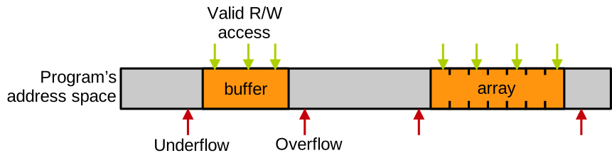
An attacker can exploit these errors to tamper with or leak sensitive data and code, execute malicious code, and disturb or crash the program – in other words, the attacker can break all aspects of the confidentiality/integrity/availability triad.
Temporal Memory Safety corresponds to the enforcement of accesses to memory while it is valid. Temporal violations happen when memory that is no longer valid because it has been deallocated, or not yet valid because it has not been initialised yet, is accessed. Below we can see an example of temporally valid and invalid memory accesses:
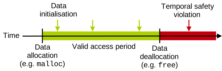
The invalid access is a use-after-free, with a buffer allocated, initialised and accessed legitimately, freed, and accessed again after the free operation. Any access past the moment free was called is a temporal safety violation. Similarly to spatial errors, temporal ones allow an attacker to break all aspects of the confidentiality, integrity, and availability triad.
Beyond Memory Safety: Undefined Behaviour
Memory errors lead the program into what is called undefined behaviour. The concept of undefined behaviour is aptly named: the C FAQ defines it as:
“Anything at all can happen; the Standard imposes no requirements. The program may fail to compile, or it may execute incorrectly (either crashing or silently generating incorrect results), or it may fortuitously do exactly what the programmer intended.”
That echoes well the “silent manifestation” aspect of memory errors we mentioned previously. Once again, the important thing to remember is that even if the program seems to run fine, if there is a memory error, then there is a problem, and it needs to be fixed. In other words, if the program misbehaves only one time out of 1000, it is not correct. As mentioned previously, the reason why the compiler/runtime does not trigger errors when these errors are present is that we want to have fast and efficient C programs.
Beyond memory errors, there are other programming mistakes that lead to undefined behaviour:
- Signed integer under/overflows
- Oversized shifts
- Passing a function as parameter to
sizeof - Casting an
int *into afloat *and dereferencing - Etc.
For more information about what may lead a C program into undefined behaviour, see this section of the C standard. Here is an example of integer overflow:
#include <limits.h>
// integer overflow: INT_MAX is the largest number that can be stored in an int
printf ("%d\n", (INT_MAX+1) < 0);
We add 1 to the maximum integer that can be stored in an int, INT_MAX, and check if the result is inferior to 0.
That should probably be false, but because we are overflowing the integer, the program misbehaves and prints that it is true.
Once again, following a memory error or any other issue leading a program into undefined behaviour, the entirety of its execution is invalid: the program must be considered as buggy and needs to be fixed, even if it seems to run fine.
Exploiting Vulnerabilities Part 1
You can access the slides 🖼️ for this lecture.
Here we are going to see how the memory safety violations we have discussed can constitute security vulnerabilities that can be exploited by attackers to subvert programs.
Memory Unsafety in C/C++
As we have seen, C and C++ are not memory safe. Programming mistakes may introduce memory errors and other bugs that are hard to detect and debug. When these bugs are present, there is often no error or warning reported at compile time, and the issue could further be completely silent at runtime. Beyond leading to program crashes or misbehaviour, these bugs can also constitute security vulnerabilities that can be exploited by attackers to break all aspects of the confidentiality/integrity/availability triad. Exploiting these bugs lets attackers leak and tamper with sensitive data, escalate privileges, take over the execution flow of programs, and disturb or crash applications and systems.
This represents a significant problem. In fact, a few years ago both Microsoft and Google reported that about 70% of their security bugs were due to memory safety violations.
Let’s have a look at a first example of a vulnerable program, where sensitive data is leaked.
Example 1: Infoleak
We assume the following scenario. We have a program that is distributed in binary-only form (that’s how most Windows proprietary applications are shipped). It contains some sensitive data: a password. An attacker has access to the binary only, not the source, and aims to figure out the password.
The program’s source originally is:
Original code:
char *welcome_message = "Hi there! How is it going?\n"; // 27 characters
char *password = "secret";
char entered_password[128];

int main(int argc, char **argv) {
    for(int i=0; i<27; i++)  // Print welcome message character by character
        printf("%c", welcome_message[i]);

    printf("Please input the password:\n");
    scanf("%s", entered_password);

    if(!strcmp(entered_password, password)) {
        printf("Password ok!\n");
        /* ... */
    } else {
        printf("Wrong password! aborting\n");
    }

    return 0;
}
The code prints a welcome message that says "Hi there! How is it going".
The message is printed character by character; it is not particularly optimal, but we need that for the sake of the demonstration.
Then it prompts the user for the password.
If the password is correct, it goes on to execute more code; if not, it prints an error message and exits.
You may already notice a very bad security practice: the password is hardcoded in plaintext in the binary.
Now imagine that the company making the program updates the code and shortens the welcome message to be "Hi there!".
The new version of the program is:
char *welcome_message = "Hi there!\n"; // shortened message, only 11 chars now
char *password = "secret";
char entered_password[128];

int main(int argc, char **argv) {
    for(int i=0; i<27; i++)           // Oopsie! forgot to update that bit of the code
        printf("%c", welcome_message[i]);

    printf("Please input the password:\n");
    scanf("%s", entered_password);

    if(!strcmp(entered_password, password)) {
        printf("Password ok!\n");
        /* ... */
    } else {
        printf("Wrong password! aborting\n");
    }

    return 0;
}
One issue here is that the programmer forgot to update the number of iterations of the loop printing the welcome message character by character. On a large and complex code base, that’s something that could happen. So now the printing loop is going to overflow the welcome message, and print on the standard output what is located in memory right after the welcome message:

At build time, when the compiler and the linker decide the layout for static memory, they will place all constant strings such as "Hi there!\n" and "secret" together in a read-only section.
The order in which constant strings are placed one after the other in that section is generally the order in which the compiler encounters them in the source code, so the chances of the password "secret" being located right after the overflowed buffer "Hi there!\n" are very high.
As a result, when the buffer is overflowed and what is past it gets printed on the command line, it is quite likely that the password itself will leak this way:
$ ./infoleak-updated
Hi there!
secretPlease inPlease input the password:
Example 2: Sensitive Data Tampering
To investigate a second example, we now assume a scenario with a similar program performing a password check, distributed as a binary only so the attacker does not have access to the sources. The attacker does not know the password and wants to bypass the password check.
Our vulnerable program is:
char user_input[32] = "00000000000";
char password[32] = "secret";

int main(int argc, char **argv) {
    if(argc != 2) { printf("Usage: %s <password>\n", argv[0]); return 0; }

    strcpy(user_input, argv[1]);
    if(!strncmp(password, user_input, strlen(password))) {
        printf("login success!\n");
        /* do important stuff  ... */
    } else {
        printf("wrong password!\n");
    }

    return 0;
}
This time the user passes the password attempt as a command line argument to the program.
That password attempt is copied into the user_input buffer with strcpy.
The content of that buffer is compared with strncmp to the correct password, and if they match the authentication succeeds.
Where is the vulnerability in this program?
Focus on the call to strcpy, as we saw previously that function will copy the entirety of the source string independently of its size.
So if the user passes to the program a password attempt whose size is larger than that of the destination buffer (32 bytes), strcpy will overflow user_input and start writing past that buffer in memory.
As in the previous program, because of how variables are declared, it is likely that the compiler will place the correct password right after the user_input buffer.
So the attacker has the ability to overwrite the correct password, by passing a string that is long enough:

This gives the attacker a write primitive in the program’s memory, i.e., the ability to set the value of both user_input and password.
If the attacker sets the content of the input it uses as a password attempt (we can call that the attack payload) in such a way that user_input and password end up having the same content, the password check will succeed:

This allows the attacker to bypass the password check:
$ ./tampering xxxxxxxxxxxxxxxxxxxxxxxxxxxxxxxxxxxxxxxxxxxx
login success!
Example 3: Stack Smashing
Let us see a third example, this time of a classic attack called stack smashing. Stack smashing lets the attacker divert the normal control flow of a program. That means the attacker can have the executed code follow paths that were not intended by the programmer. This attack was first described in 1996 in an article that has become quite famous since then. To understand stack smashing, we will first refresh our mind on how the CPU handles function calls and returns at runtime.
Assume we have the following scenario: a C program with a function f calling another function g.
In memory, when f runs, its local variables and parameters are located in its stack frame.
When f calls g, the CPU issues a call instruction.
That instruction pushes on the stack the return address of g in f: it is the address, in the code segment of the program, of the instruction that should be executed next when we will return from the call to g within f:
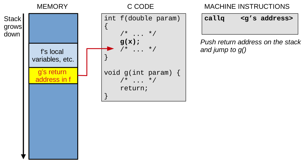
After the call g starts to run, and there is some space allocated on the stack for its own local variables and parameters.
When g returns, the CPU executes a ret instruction.
ret will pop the return address from the stack and jump to it: in this way, the execution in f resumes right after the call to g:
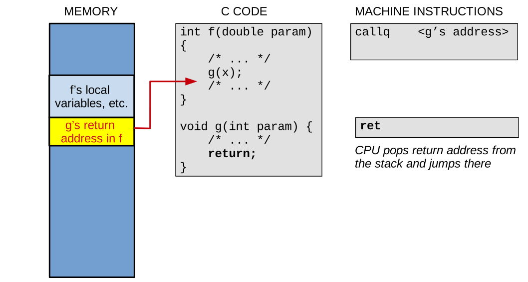
We now consider this vulnerable program:
char *password = "secret";

void security_critical_function() { printf("launching nukes!!\n"); }

void preprocess_input(char *string) {
    char local_buffer[16];
    strcpy(local_buffer, string);
    /* work on local buffer ... */
    return;
}

int main(int argc, char **argv) {
    if (argc != 2) { printf("usage: %s <password>\n", argv[0]); return -1; }

    preprocess_input(argv[1]);

    if(!strncmp(password, argv[1], strlen(password)))
        security_critical_function();
    else
        printf("Unauthorized user!\n");

    return 0;
}
It is the same type of password checking application we have seen previously.
It takes the password attempt from the command line, and before performing the check it passes it to a function named preprocess_input.
preprocess_input copies the attempt into a local_buffer before working on it.
In the code you can also see the function executed when the authentication succeeds, it is called security_critical_function.
Here the goal of the attacker is to run this function without going through the password check.
As you can see the strcpy in preprocess_input takes as source something coming from the command line, so similarly to the previous example we have the capacity to overflow local_buffer.
How can we exploit that to bypass the password check?
When preprocess_input runs, the stack looks as follows:
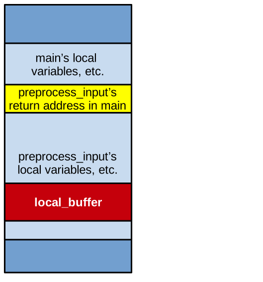
We have main’s stack frame, next we have the return address where we should jump in main when preprocess_input returns, and then we have preprocess_input’s stack frame.
local_buffer is somewhere in preprocess_input’s frame, so when we overflow it with strcpy, we have the ability to overflow upwards in the stack, towards the high addresses:
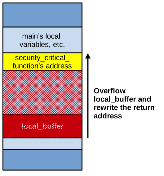
If we craft the content of what we overflow local_buffer with carefully, we can make it in such a way that we overwrite the return address with the address of our target, which is security_critical_function.
Doing so, when preprocess_input returns, the CPU will pop our overwritten return address on the stack and jump to it:
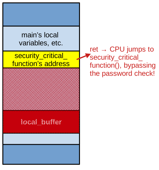
In effect, the CPU will start executing security_critical_function without going through the password check.
See the complete program’s sources here for instructions on how to reproduce this attack. On the computer on which this code was tested, the payload (injected with echo -e and xargs to produce bytes and not ASCII characters) looks like this:
$ echo -e "\x11\x11\x11\... (24 bytes of \x11 padding) ... \x5e\x17\x40\x00\x00\x00\x00\x00" \
    | xargs --null -t -n1 ./stack-smashing
./stack-smashing ''$'\021\021\021\021\021\021\021\021\021\021\021\021\021\021\021\021\021\021
    \021\021\021\021\021\021''U'$'\026''@'
launching nukes!!
xargs: ./stack-smashing: terminated by signal 11
Example 4: Use-After-Free
So far we have seen how spatial memory errors (buffer overflows) can be exploited to various effects. We now examine an example of exploitation of a temporal memory error: a use-after-free.
This is our vulnerable program:
typedef struct {
    double member1; double member2;
    void (*member3)(int);
} my_struct;

void print_hello(int x) {
    printf("Hello, parameter: %d\n", x);
}

void security_critical_function() {
    printf("Launching nukes!\n");
    /* ... */
}

int main(int argc, char **argv) {
    /* allocate and init ms */
    my_struct *ms = malloc(sizeof(my_struct));
    ms->member1 = 42.0; ms->member2 = 42.0;
    ms->member3 = &print_hello;
    /* call the function pointer */
    ms->member3(12);

    free(ms);
    char *buffer = malloc(12);
    strcpy(buffer, argv[1]);

    ms->member3(12);

    /* check a password, runs sec_crit_fn */
}
It declares a data structure my_struct for which one of the members, member3, is a function pointer.
In main a data structure object ms is allocated with malloc and initialised, with the function pointer set to point to a benign function that prints a welcome message.
The object is then freed, then there is another call to malloc and the buffer in question is filled with data from the command line arguments, with strcpy.
And then finally we have our use-after-free: the object ms, previously freed, is mistakenly accessed: the function pointer is dereferenced.
We also have a security-critical function, and the goal of the attacker is to redirect the execution of the program to that function without going through a password check.
We now examine how we can exploit this program.
When the object ms is initialised, the memory layout looks as follows:
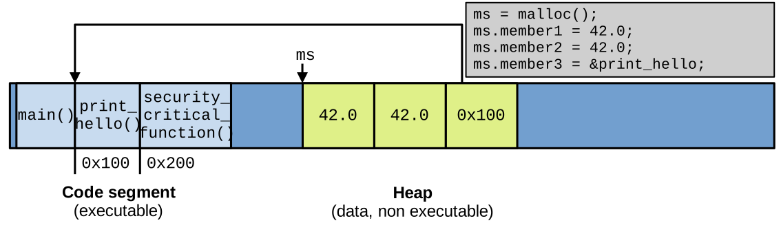
The 3 members of the object are laid out contiguously in memory, and the function pointer points to the first byte of code of the print_hello function in the code segment.
When free is called that memory is discarded:
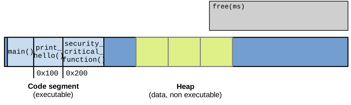
Due to the way malloc is implemented, it will try to reuse freed memory for future allocations as much as possible.
So it is likely that the space that previously held the ms data structure will be reused for the next allocation, which is filled with data coming from the command line parameter:
With strcpy the attacker can write in that space, and overflow the 12 bytes of buffer to overwrite the space that previously held the function pointer with the address of security_critical_function:
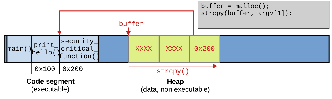
Later when the use-after-free happens, this in effect invokes the security_critical_function.
Please see the full source code for instructions on how to reproduce that attack. On the computer on which this code was tested, the payload looks like this:
$ echo -e "\x11\x11\x11\ ... (16 bytes of \x11 padding) ... \x7c\x16\x40\x00\x00\x00\x00\x00" \
    | xargs --null -t -n1 ./use-after-free
./use-after-free ''$'\021\021\021\021\021\021\021\021\021\021\021\021\021\021\021
    \021''|'$'\026''@'
Hello, parameter: 12
Launching nukes!
# program continues to misbehave after that
Advanced Control Flow Hijacking
The last two examples of attacks we have seen are named control flow hijacking attacks: the attacker diverts the control flow of the program and has the CPU run code paths that are different from what the programmer originally intended.
Concretely, our examples showed how the attacker can rewrite return addresses and function pointers to return and jump to security-critical pieces of code.
Other control flow hijacking attacks can attempt to jump to C standard library functions, for example jumping to the exec function while having the string "/bin/sh" in the register holding the first function parameter according to the ABI can lead to a remote attacker getting access to a shell on the victim machine.
Another relatively advanced attack is named return oriented programming (ROP). With ROP, the attacker has full control over what is on the stack, for example through an overflow. The attacker places on the stack a series of code addresses that point to small snippets of machine code. These are called gadgets, and represent sequences of just a few instructions ending with ret. In this way, the CPU executes the first sequence of instruction, returns to the second, executes it, then returns to the third, and so on:
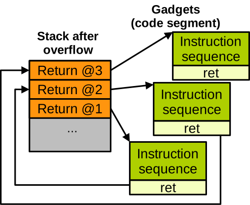
In modern programs there is a very high number of gadgets in the code segment. In fact, on medium to large size programs, the attacker can generally achieve Turing complete computations through ROP, which makes it a particularly concerning attack vector.
Exploiting Vulnerabilities Part 2
You can access the slides 🖼️ for this lecture.
Here we discuss the concept of trust boundaries in programs.
Distrusting Command Line Parameters
In most of the examples of attacks we covered previously, the payload was coming from the command line. As a reminder, the payload is the malformed piece of program input that the attacker uses to trigger a vulnerability and perform an exploit. Not trusting the validity of the number and the values of command line parameters is a well-known security practice when developing systems software.
In fact, now that we are talking about distrusting some forms of input to the program, we can try to reason about what our trust model was for all these attack examples we saw. From the victim’s program protection point of view, we trust the privileged layers like the OS, as well as the hardware, to work correctly. What we did not trust was other programs that could inject command line arguments into our victim program. If the program is invoked by the attacker on the command line, as we have seen in our examples, this untrusted other program could be the invoking shell. Our trust model can be illustrated as follows:
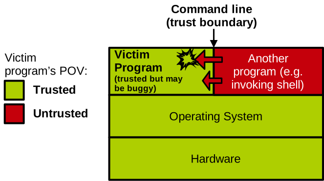
It is well known that a programmer should never assume that any data flowing into the program through command line arguments is well-formed. To trigger vulnerabilities, an attacker can try to invoke the program with the wrong number of command line parameters, a bad combination of parameters, or invalid types, sizes, or ranges for certain parameters. As the developer of an application, it is important to reason about how the program reacts when something malformed is passed through the command line. Will the program crash or misbehave? If so, that is not good, and we are probably looking at security issues as we have seen in the previous examples. The proper way to deal with these malformed program inputs is to handle them gracefully, for example by printing an error message and exiting the program.
Please also note that this is not just about a well-intentioned user invoking the program and setting by mistake the wrong number of arguments or the wrong value for an argument. The programmer needs to reason about the target trust model, and assume that untrusted actors will actively try absolutely anything possible to trigger bugs in the program to subvert it.
Trust Boundaries in Programs
The command line in our scenario is an interface between a trusted (program) and an untrusted component (external environment, e.g., invoking shell): it’s a trust boundary. That makes this interface a vector of attack: protection is required to ensure that all the data flowing through this interface is valid before it can be used by the trusted component. This protection needs to be implemented by the programmer and consists of a series of sanity checks. Examples of such sanity checks are:
- Do we have the right amount of parameters?
- Do parameters make sense together (proper combinations)?
- Do parameters have proper values in terms of types, ranges, format, etc.?
Beyond the command line parameters, there are several other common sources of untrusted input in modern systems software
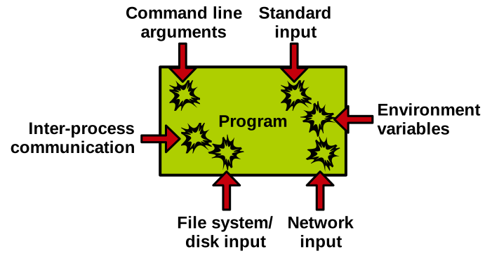
- The standard input can be used by an attacker to feed bad data to your program.
- Environment variables can be manipulated.
- All the data flowing into the program through disk or network I/O could be invalid: malformed file formats, corrupted network packet data/metadata, etc.
- Finally, if the application we aim to secure is communicating with another program that is not trusted through inter-process communication, that is also a vector of attack.
Which of these attack vectors to consider in order to secure an application depends on the target threat model, but almost every production-ready program using these interfaces will need to perform sanity checks on the data flowing through them.
Example: Command Line Arguments
We have already seen plenty of examples of programs that can be subverted through malformed command line arguments. Here we have a vulnerable program with two buffers that can be overflown:
#include <stdio.h>
#include <string.h>

// usage: ./cmdline <username> <password>
int main(int argc, char **argv) {
    char username[32];
    char password[32];

    strcpy(username, argv[1]);
    strcpy(password, argv[2]);

    // ...
}
A protected version of that program is as follows:
#define USERNAME_MAX_LEN    32
#define PASSWORD_MAX_LEN    32

int main(int argc, char **argv) {
  char username[USERNAME_MAX_LEN];
  char password[PASSWORD_MAX_LEN];

  // check the number of parameters
  if(argc != 3) {
      printf("usage: %s <uname> <passwd>\n",
        argv[0]);
      return 0;
  }

  // don't copy past the buffer size
  strncpy(username, argv[1], USERNAME_MAX_LEN);
  strncpy(password, argv[2], PASSWORD_MAX_LEN);

  // make sure strings are properly terminated
  username[sizeof(username) - 1] = '\0';
  password[sizeof(password) - 1] = '\0';
  // ...
}
As we can see, we first validate that we have the right number of command line arguments.
Then, with strncpy, we make sure not to copy more bytes than the size of the receiving buffers.
And finally we make sure that the strings are properly terminated, because the attacker could pass them in such a way that they are not.
Example: Environment Variables
Here is another example of bad data injection, this time through an environment variable:
#include <stdio.h>
#include <stdlib.h>

// usage: USER_INPUT=pierre ./environment-variable
int main(int argc, char *argv[]) {
    char *user = getenv("USER_INPUT");
    if (!user) {
        fprintf(stderr, "Please set the USER_INPUT environment variable.\n");
        return 1;
    }

    char buffer[100];

    // Vulnerable: format string comes from environment variable
    snprintf(buffer, 100, user);

    printf("Hello, ");
    puts(buffer);

    return 0;
}
We first get a pointer to the value of this environment variable named USER_INPUT with the getenv libc function.
Then we use snprintf to copy the value of the environment variable into buffer.
There is no possibility of overflow here, because we know that snprintf won’t write more than 100 bytes which is the size of the receiving buffer.
However, snprintf takes as its third parameter a format string, and optionally as fourth and subsequent parameters a list of variables whose values should be substituted for tokens in the format string, exactly like printf.
So if we pass through the environment variable something that looks like a format string with tokens, we can leak part of the program’s memory on the command line when the format string is printed:
$ gcc environment-variables.c -o environment-variables
$ USER_INPUT="%p %p %p %p %p %p" ./environment-variables
Hello, 0xa 0xffffffff (nil) 0x7ffc34723608 0x100000040 0x2000000
Some of these look like pointers, and leaking pointers is an important step in many attacks as we will see next in this unit.
The fix to get rid of the vulnerability is simple: have the format string be simply %s, and have that token be replaced by snprintf with a single variable which is the value of the environment variable:
#include <stdio.h>
#include <stdlib.h>

// usage: USER_INPUT=pierre ./environment-variable
int main(int argc, char *argv[]) {
    char *user = getenv("USER_INPUT");
    if (!user) {
        fprintf(stderr, "Please set the USER_INPUT environment variable.\n");
        return 1;
    }

    char buffer[100];

    snprintf(buffer, sizeof(buffer), "%s", user);

    printf("Hello, ");
    puts(buffer);

    return 0;
}
If we try the attack it does not succeed:
$ gcc environment-variables-fixed.c -o environment-variables-fixed
$ USER_INPUT="%p %p %p %p %p %p" ./environment-variables-fixed
Hello, %p %p %p %p %p %p
Even simpler: for copying a string just use strncpy.
Example: HeartBleed
Let’s have a look at one last example, this time taken from the real world. You may have heard about the HeartBleed vulnerability (CVE-2014-0160) in the OpenSSL library that is used to encrypt most of the HTTPS traffic of the internet. It’s a very severe issue that caused a big commotion in 2014.
With HeartBleed the attacker’s payload comes through the network. The attacker here controls a remote client and aims to leak sensitive data from the server. The client regularly sends a heartbeat request to the server to keep the connection alive. The client indicates within the request the size of the response the server should send back, and sets that number to a larger value than the actual response the server will write. This triggers a read overflow on the heap of the server, and the memory read this way is sent back to the client. It could contain anything, including crypto keys that are commonly manipulated by that library.
An excellent illustration of the HeartBleed bug is presented in this xkcd comic.
Under normal operation the client asks the server to respond with POTATO and also gives the server the size it should use to respond, which is 6 letters: the server then answers POTATO in 6 letters and all is well.
The client repeats the process, this time with BIRD in 4 letters, and things work as expected.
The exploit consists in the client asking the server for a relatively small reply but with a very large reply size: here the reply should be BIRD, but rather than specifying a size of 4, the client requests 500 letters.
This leads to a read overflow in the server’s memory, of a bit less than 500 bytes past the buffer holding BIRD.
This memory is sent back to the client, and it may contain very sensitive data due to the security-critical nature of the OpenSSL library.
Here is a simplified implementation of the HeartBleed bug in the code of the server:
int main() {
    char secret[64] = "SECRET: This is private data that shouldn't leak!\n";
    int server = socket(AF_INET, SOCK_STREAM, 0);
    int opt = 1;
    setsockopt(server, SOL_SOCKET, SO_REUSEADDR, &opt, sizeof(opt));

    struct sockaddr_in addr = { .sin_family = AF_INET, .sin_port = htons(12345),
        .sin_addr.s_addr = INADDR_ANY
    };

    bind(server, (struct sockaddr*)&addr, sizeof(addr));
    listen(server, 1);

    int client = accept(server, NULL, NULL);

    unsigned char buf[32] = {0};
    recv(client, buf, sizeof(buf), 0);

    // Heartbleed-style vulnerability:
    // client sends: [type][len][data] -> respond with `len` bytes
    int len = buf[1];  // vulnerable: no bounds check
    send(client, buf + 2, len, 0);

    close(client); close(server);
}
You can see that the server receives data from the client in a 32-byte buffer, according to a particular format. The first byte indicates the request type, used to indicate a heartbeat request. The second byte indicates the size the server response should have, and the next 30 bytes contain the data that should be present in the server’s response.
We can reproduce the exploit by compiling and launching the server in a terminal:
$ gcc heartbleed.c -o heartbleed
$ ./heartbleed
And sending the payload to the server from another terminal with Netcat:
$ printf '\x01\x90hi' | nc localhost 12345
hiSECRET: This is private data that shouldn't leak!
P%��(�
7�nh%��N|�a���a����U%%
What matters here is the second byte of the payload (0x90, which is 144 in base 10) followed by a message whose size is much smaller than 144 bytes: hi.
So the vulnerable server overflows buf on the stack and sends to the client the overflowed content, which happens to include the secret.
The fix is simple: put a cap on the size that can be indicated by the client. Here we make sure it cannot be longer than the 30 bytes we have to hold it:
int client = accept(server, NULL, NULL);

unsigned char buf[32] = {0};

// zero out buf:
memset(buf, 0x0, 32);

recv(client, buf, sizeof(buf), 0);

int len = buf[1];

// sanity check len:
if(len > (32-2))
    len = (32-2);

send(client, buf + 2, len, 0);
Handling Trust Boundaries
So, as we saw, it’s very important that, as a developer, you secure the trust boundaries in your program. For that, you need to reason about your trust model. Here is an example of a trust model for a server:
| Source | Example Use | Trust Level | Reasoning / Risk |
|---|---|---|---|
| Command-line arguments | ./server --config=config.txt | ❌ Untrusted | User-controlled; could point to malicious files or overflow buffer sizes |
| Environment variables | export PORT=8080 | ❌ Untrusted | Inherited from shell; attacker can manipulate via scripts or misconfigurations |
| Standard Input | Admin enters reload via terminal | ❌ Untrusted | Human error or input injection if stdin is redirected |
| Configuration file | Parses config.txt for allowed IPs or auth keys | ⚠️ Partially trusted | Could be modified by external actors; needs file integrity checks and format validation |
| Network input | Receives GET /index.html requests via TCP socket | ❌ Totally untrusted | Malicious clients can send malformed, oversized, or malicious payloads |
| Internal constants | Default port = 80, buffer sizes | ✅ Trusted | Controlled by developer; no user influence |
We do not trust the command line arguments or environment variables. If there is somehow an interactive command line, we do not trust whatever comes through the standard input either. We do not trust network input either; requests could be malformed, as we just saw. The server’s configuration files on the filesystem are partially trusted: it may be possible for an attacker to alter them if the filesystem permissions are not set up correctly, so a bit of sanity checking on the configuration coming from these files is probably a good idea. Finally, internal constants in the program’s binary are assumed to be trusted.
Based on a defined trust model, it is the developer’s responsibility to identify interfaces between untrusted and trusted components, and to sanity check all the data and control flow going through these interfaces. That means validating, before use, data types, sizes, ranges, but also the consistency of pieces of data together. It also allows avoiding leaking data and references to untrusted components by zeroing out data that is not initialised.
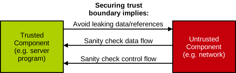
But it is not only about data: the control flow should be validated too. An example here is enforcing ordering: if a networked application defines a communication protocol with another untrusted program, and the protocol requires that requests of type A should always be sent before requests of type B, what are the implications of the untrusted program sending B before A?
Securing such interfaces becomes very hard when the program and its trust boundaries are large and complex. This is why we have entire classes of software that are quite prone to suffer from vulnerabilities, because it is impossible to guarantee that their trust boundaries have been 100% sanitised:
- Parsers, that handle feature-rich and complex (e.g. XML) formats;
- Web browsers, handling large amount of untrusted inputs (e.g. HTML, CSS, JS, etc.);
- Image/document processors, processing complex file formats, sometimes embedding code;
- Shell/command line parsers that may support many features;
- Network protocol stacks, that can be complex and support many features/types of requests;
- Etc.
All of these are complex pieces of software handling complex data formats, often exposing interfaces that are themselves proportionally complex.
Secure Coding Practices, Detecting Bugs
You can access the slides 🖼️ for this lecture.
Here we review methods to try to minimise the number of bugs we introduce when writing systems software.
Context
We have seen that memory safety and undefined behaviour issues are common in systems software, and that they lead to security vulnerabilities that can be exploited by attackers to compromise the confidentiality, integrity, and availability of systems software. How can we address that problem? In practice, we can do three things:
- When we develop we need to adhere to good coding practices to minimise the chances of introducing such bugs.
- We have techniques that can help analyse our code during development and detect some bugs.
- We also have techniques that can help protect programs in production, making exploitation more difficult and limiting the damage from successful exploits.
Here we discuss 1 and 2, and the next chapter will cover 3.
Good Coding Practices
As we have seen, the memory errors and other sources of undefined behaviour that lead to security vulnerabilities come from programming mistakes. When developing systems software, how can we avoid introducing these programming mistakes as much as possible? There are two main aspects to this problem:
- First, how to avoid introducing these programming mistakes when writing code?
- Second, how to detect these programming mistakes in existing code?
We cover both aspects next, starting with secure coding practices.
Array/Buffer/Integer Overflows
To prevent array or buffer overflows, you need to know their sizes: you must be aware of the size of an array to know when to stop iterating over it, and of the size of a destination buffer to know how many bytes you can write in there. In C, recall that arrays and buffers do not embed their sizes, so make sure to keep track of the size of each array/buffer you use.
When manipulating integers, make sure to be aware of the size reserved by the compiler to hold them in memory according to the architecture you are compiling for, in order to avoid overflows.
You can use sizeof to determine these sizes.
An unsigned integer will never overflow but rather wrap around; overflowing a signed integer leads to undefined behaviour and must be avoided.
The compiler has some built-in functions that can tell you if an integer operation overflows.
These operations are available for integer addition, subtraction, and multiplication.
C Standard Library Functions
Unsafe Functions to Avoid. Here are a few functions of the libc whose use should be avoided as much as possible:
| Unsafe Function | Why It Is Unsafe | Safe Alternative(s) |
|---|---|---|
gets() | No bounds checking; allows buffer overflows | fgets() |
strcpy() | No bounds checking; can overflow destination buffer | strncpy(), strlcpy() (if available) |
sprintf() | No bounds checking; leads to buffer overflows | snprintf() |
scanf() | No bounds checking e.g., %s with no width | fgets() + sscanf() with width specifiers |
memcpy() | No bounds checking; can cause overflows | Use with care; consider memmove() for overlapping memory |
bcopy() | Obsolete; unsafe due to no bounds checking | memmove() |
strlen() | Not inherently unsafe, but must not be used on untrusted or unterminated buffers | Ensure string is null-terminated before use |
The table explains the reason why each function is unsafe, as well as safe alternatives.
Several of them, such as strcpy, have no bounds checking, hence no way to prevent overflows.
You should use the safe versions of these functions as much as possible, which all have a way to indicate the size of the receiving buffer to avoid overflows.
To move memory you should not rely on bcopy but rather use memcpy (with care, i.e. you have to handle bounds checking) if the source and target areas do not overlap, and memmove if they do.
Finally, be careful with strlen: it can return numbers larger than the size of a string if that string is not properly terminated.
These are not the only functions to avoid; please see here for more.
String Manipulation Functions.
Once again, regarding string manipulation functions, careful developers should use the n versions that require indicating a maximum number of characters to process: strncpy rather than strcpy, snprintf instead of sprintf, etc.
Even with the versions with n, there are some particularities to keep in mind, for example strncpy will not add the termination character \0 at the end of the target buffer.
Consider this code in which we wish to replace the content of string2, that is composed of 32 x’s, with "hello, world".
char string1[] = "hello, world";
char string2[32] = "xxxxxxxxxxxxxxxxxxxxxxxxxxxxxxx";

strncpy(string2, string1, strlen(string1));
printf("%s\n", string2); // prints "hello, worldxxxxxxxxxxxxxxxxxxx"
Because strncpy does not add the termination character, we end up with a mix of both strings which is probably not what the programmer intended.
Dynamic Memory Allocation
When using dynamic memory allocation, make sure to always check malloc’s return value, for reasons we have previously discussed.
Also remember that, after free is called upon a pointer, that pointer is invalid and should not be reused in any way.
It should obviously not be dereferenced, but its value should not be used for any other purpose.
As we have seen previously, realloc returns NULL upon failure but does not free the old pointer, so the following code is in effect a memory leak:
ptr = realloc(ptr, new_size);
malloc does not zero out memory returned to allocation requests, so if you only partially initialise a data structure located in a dynamically allocated buffer, and you pass that data structure to a context that you do not trust (for example by sending it through the network), you may be leaking memory content to that untrusted party.
So for buffers sent to untrusted contexts, it is better to use calloc, which will zero out the memory it allocates, at the cost of a performance slowdown.
Secure Coding: Further Readings
What we have seen is just a few examples of secure coding practices, and we do not have time to cover them all exhaustively. You can see on the slides a list of good resources; make sure to check them out if you want to learn more:
- SEI CERT C Coding Standard: https://wiki.sei.cmu.edu/confluence/display/c
- Robert C. Seacord, Secure coding in C and C++ (book)
- ISO/IEC TS 17961 (C Secure Coding Rules): https://www.open-std.org/jtc1/sc22/wg14/www/docs/n1624.pdf
- NASA JPL C Coding Standard: https://yurichev.com/mirrors/C/JPL_Coding_Standard_C.pdf
- Fedora’s Defensive Coding Guide: https://docs.fedoraproject.org/en-US/defensive-coding/
Detecting Coding Mistakes
Let’s now investigate analysis tools that can help detect programming mistakes and vulnerabilities in existing code. Here we will cover techniques that are slow to execute, or that make the application slow. As a result, they cannot run in production, and are rather used during development, often integrated with applications’ CI/CD pipelines.
These techniques fall within two main categories:
- Static analysis approaches
- Dynamic analysis approaches
Static Analysis
Static analysis tools scan the source code of a program for possible bugs without actually running the program. An important benefit of this approach is that it has good coverage: it analyses the entire program’s code, which lends itself well to automation. In terms of downsides, static analysis generally suffers from false positives: this means it may identify issues in the code that actually do not represent programming mistakes or security vulnerabilities. Because it does not run the program, static analysis also operates with limited context: for example, much of the memory’s content is not determined until runtime. Finally, some static analysis techniques are quite slow, and do not scale well to the large code bases of certain systems software.
Compiler Warnings and Errors. A first form of static analysis is compiler warnings and errors. A careful programmer should enable high degrees of compiler warnings. The compiler flags that can be used are, in increasing order of strictness:
-Wallto get additional warnings.-Wextrato get even more warnings.-pedanticto add even more warnings.
High degrees of strictness may yield a high number of false positives.
The -Werror flag will transform warnings into errors: the first warning encountered will stop the compilation process, forcing the programmer to fix it to be able to build the program.
To understand what types of warnings are added by each option, see GCC’s relevant documentation.
Code Static Analysis Tools. There are many advanced static analysis tools; a few examples are:
Next, we present an example of using the Clang static analyser. Consider the faulty program below; it contains three bugs:
int c;

int main() {

    int a = INT_MAX;
    int b = 1;
    c = a + b; // Integer overflow!

    char buffer[8];
    char str[] = "this string is too long";
    strcpy(buffer, str); // Buffer overflow!


    int *ptr = (int *)malloc(sizeof(int));
    *ptr = 42;
    free(ptr);
    *ptr = 99; // Use-after-free!

    return 0;
}
The first bug is an integer overflow: c’s value is set to the largest integer that can be stored in an int, INT_MAX, then it is incremented, which triggers the overflow.
The second bug is a buffer overflow: we copy into buffer (whose size is 8 bytes) a string str that is larger than 8 bytes.
And the last bug is a use-after-free, where we dereference the pointer ptr after freeing the memory it points to.
Notice that with the default level of warnings, this program compiles fine, and also it runs without any visible error:
$ gcc faulty.c -o faulty
$ ./faulty
Let’s see if the bugs it contains can be detected with the Clang static analyser. To run the analyser, invoke it as follows:
$ clang --analyze faulty.c
faulty.c:22:10: warning: Use of memory after it is freed [unix.Malloc]
    *ptr = 99; // Use-after-free!
    ~~~~ ^
1 warning generated.
The analyser detects the use-after-free, which is good. However, it does not identify the integer and buffer overflows. For that we need to rely on the second main class of analysis tools: dynamic analysis.
Dynamic Analysis
Dynamic analysis tries to detect errors while running the program. By doing so, it gets access to more information than static analysis, that is runtime information (for example the content of memory or the value of program input). Dynamic analysis is also useful when the sources of the program we wish to analyse are not available (black-box testing).
A very popular type of dynamic analysis is achieved through compiler-based instrumentation: at build time the compiler inserts additional instructions in the program to detect bugs later at runtime. The code sanitisers are a series of tools enabling such dynamic analysis. The most widespread is address sanitiser (ASan). ASan will detect a wide range of memory errors that would not be caught at compile-time or at runtime without the instrumentation. We also have the undefined behaviour sanitiser (UBSan), that detects things like integer overflows, invalid casts, and so on, or the thread sanitiser, that will detect concurrency issues such as race conditions.
More information on code sanitisers is available here.
Sanitisers: ASan and UBSan. We can illustrate the use of ASan and UBSan by running these analysis tools on our faulty program. To instrument the program with ASan, compile it as follows:
$ clang -fsanitize=address faulty.c -o faulty
Then simply launch the program normally:
$ ./faulty
=================================================================
==21543==ERROR: AddressSanitizer: stack-buffer-overflow on address 0x7ffcc881f268
...
As one can see, ASan can catch the buffer overflow. Once that buffer overflow is fixed, we can recompile, still with ASan enabled, and re-run the analysis:
clang -fsanitize=address faulty.c -o faulty
$ ./faulty
./faulty
=================================================================
==22504==ERROR: AddressSanitizer: heap-use-after-free on address 0x602000000010 # ...
This time we can see that the use-after-free is detected. We can also enable UBSan:
$ clang -fsanitize=undefined faulty.c -o faulty
$ ./faulty
faulty.c:12:11: runtime error: signed integer overflow:
    2147483647 + 1 cannot be represented in type 'int'
UBSan successfully detects the integer overflow.
Valgrind. There are other dynamic analysis tools beyond the sanitisers, although many of such tools have been rendered more or less obsolete by them. We have seen Valgrind previously. In addition to reporting memory leaks, it can also detect certain memory errors. Given that sanitisers also detect memory leaks, that makes Valgrind quite redundant. However, one benefit over sanitisers is that Valgrind does not require recompiling the program to insert instrumentation. Hence, Valgrind is still useful in contexts where we have access only to the application’s binary and not its sources (e.g., black-box testing of proprietary software).
Fuzz-Testing. A highly popular modern dynamic analysis technique is fuzzing (sometimes referred to as fuzz-testing). It consists in blasting a trust boundary with malformed inputs (e.g., pseudo-random data) with the hope of triggering bugs. Examples of trust boundaries that are good candidates for fuzzing include command-line arguments, input files, network packets, and so on. Fuzzing is widespread today, and this technique helps uncover a very large number of bugs in many projects.
Let’s see an example of fuzzing with the tool American Fuzzy Lop (AFL). We will fuzz the following vulnerable program:
int main(int argc, char *argv[]) {
    char name[32];  // Vulnerable buffer (too small for unchecked input)

    if (argc < 2) {
        printf("Usage: %s <input file>\n", argv[0]);
        return 1;
    }

    FILE *f = fopen(argv[1], "r");
    if (!f) {
        printf("Error, can't open %s\n", argv[1]);
        return 1;
    }

    fread(name, 1, 512, f);  // Reads up to 512 bytes into a 32-byte buffer!
    fclose(f);

    printf("hello %s\n", name);
    return 0;
}
This program opens a file and reads its content into a buffer. It reads 512 bytes; however, the destination buffer is only 32 bytes long, so there is a possibility of overflow here. The name of the file to read comes from the command line. We are going to fuzz this program by invoking it repeatedly and injecting files with random data and variable sizes, which should help trigger the bug.
To install AFL on an Ubuntu/Debian distribution:
$ sudo apt install afl # or afl++ on very recent ubuntu/debian distributions
We first need to compile and instrument our target program for fuzzing:
$ afl-clang fuzzme.c -o fuzzme
In addition to inserting the necessary code for fuzzing, the instrumentation will also enable sanitisers to maximise the number of bugs discovered. Before being able to fuzz, we also need to create a seed input to help kickstart the fuzzing process:
$ mkdir input
$ echo "testname" > input/seed
Finally, we can start the fuzzing process as follows:
$ AFL_SKIP_CPUFREQ=1 afl-fuzz -i input -o output -- ./fuzzme @@
AFL’s window will report, in real time, statistics about the fuzzing process: runtime, number of program invocations, fuzzing strategy used, and so on.
Pay attention in particular to the total crashes : field: there should be at least one crash discovered very quickly after the start of the fuzzing process.
Crashes represent potential bugs (e.g., ASan crash) found by the fuzzer.
By default, AFL will fuzz indefinitely: to terminate the fuzzing process, hit ctrl+c on the keyboard.
To reproduce manually a particular crash uncovered by the fuzzer, compile the program normally with ASan enabled, and inject the payload corresponding to that crash:
$ clang -g -fsanitize=address fuzzme.c -o fuzzme
$ ./fuzzme output/crashes/id:000000,sig:11,src:000000,op:havoc,rep:128
...
==161882==ERROR: AddressSanitizer: stack-buffer-overflow on address 0x7b2b61bf0040 at pc 0x559b133ffbac bp 0x7ffc92be10f0 sp 0x7ffc92be08b0
WRITE of size 36 at 0x7b2b61bf0040 thread T0
    #0 0x559b133ffbab in fread.part.0 asan_interceptors.cpp.o
    #1 0x559b13531ff0 in main /home/pierre/Desktop/comp60261/slides/10-secure-coding-practices-detecting-bugs/src/fuzzme.c:20:5
...
Note that the name of the payload file may be different on your computer. As one can see, the payload successfully triggered the buffer overflow present in our buggy program.
There is a lot more to say about fuzzing. It’s a field that has seen a lot of recent developments. A few relevant further readings:
Other Static and Dynamic Analysis Approaches. There are a few other static and dynamic analysis techniques that can be used to detect programming mistakes, bugs, and vulnerabilities. You are probably familiar with unit testing and manual code reviews, as well as with tools to check that code follows a certain style (linters/style checkers). There are other advanced techniques that we won’t cover here, but have shown good results:
Runtime Defences
You can access the slides 🖼️ for this lecture.
Here we discuss defences running at runtime in production.
Non-Executable Memory
In the past, a large part of the address space used to be accessible with execution right. That was quite detrimental from the security point of view: it meant that an attacker armed with a memory write primitive (e.g., as we have seen following a buffer overflow) could write malicious machine code in a memory area that is both executable and writable, and then have the CPU jump to it: that is called a code injection attack.
In the early 2000s, hardware support appeared to tackle that issue by setting part of the address space as non-executable. Such hardware was used to set everything that should not be accessed in executable mode as non-executable: the stack, heap, static data sections, etc. This can be illustrated as follows:
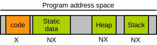
This is an application of the principle of least privilege, and it made code injection attacks much less likely. Today, setting memory as non-executable is generally achieved through a specific bit in each page table entry, controlling the executable/non-executable status of the memory page it corresponds to: the NX bit.
Today, modern systems software aim to enforce the “write xor execute” (W⊕X) principle for each memory area: that principle states that you cannot have an area of memory be both writable and executable at the same time.
Address Space Layout Randomisation
Another defence that is present in almost every system today is address space layout randomisation (ASLR). With ASLR, each invocation of the program will have a different layout for the address space. In other words, code and variables will not be at the same location in memory for subsequent invocations. The goal is to make it harder for the attacker to determine what is where in the address space. Recall from the attacks we have seen previously that many of them require us to know exactly where a buffer to overflow is present or the stack, or exactly where we need to jump in the code segment. This is achieved by observing one invocation of the program, for example with a debugger, and then starting the attack upon a second invocation of the program. With ASLR that will not be easy to achieve because the locations of the data and code we determine with the first invocation are not the same for the second:
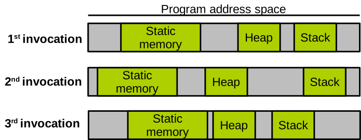
Note that the granularity of ASLR in most production systems is coarse: for performance reasons we cannot really randomise the location of each variable independently. Hence, randomisation is realised at the level of a program’s entire segments, as illustrated above. It is realised at load time for the main program, and when dynamic libraries are loaded.
To understand the security implications of coarse-grained ASLR, consider the following program:
int global1 = 42;
int global2 = 43;

int main() {
  int local1 = 24;
  int local2 = 25;

  int *heap_ptr1 = malloc(sizeof(int));
  int *heap_ptr2 = malloc(sizeof(int));

  printf("data addr 1: %p\n", &global1);
  printf("data addr 2: %p\n", &global2);
  printf("stack addr 1: %p\n", &local1);
  printf("stack addr 2: %p\n", &local2);
  printf("heap addr 1: %p\n", heap_ptr1);
  printf("heap addr 2: %p\n", heap_ptr2);

  free(heap_ptr1);
  free(heap_ptr2);
}
This code simply prints the addresses of two local variables, two global variables, and the value of two heap pointers. We observe that:
- The relative distance between two variables located in different segments is randomised across different invocations of the program.
- The relative distance between two variables belonging to the same segment stays the same across executions.
This is because only the base address of each segment is randomised at load time. As a result, if an attacker can leak the value of a single pointer, it is easy for them to compute the address of all other data or code within the containing segment. Hence, the coarse-grained nature of ASLR on modern systems makes it relatively easy to break.
Stack Canaries
The stack canary is a technique protecting the return address on the stack from being overwritten by attackers. The key idea is to place a magic value named the canary right before the return address in a callee’s stack frame, to compare that canary’s value to a ground truth when the callee returns. In practice, stack canaries work as follows:
At build time, the compiler inserts code to place the canary on the stack right after the return address upon each function call:
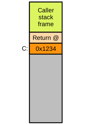
In our example the canary’s value is 0x1234.
At build time the compiler also inserts code to check that the canary still contains the correct value upon each function return:
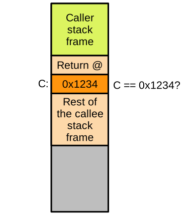
At runtime, a canary value is inserted upon each function call, and its value checked when that function returns. Should an attacker attempt a stack smashing attack through a stack buffer overflow vulnerability as we described previously, the overflow will overwrite the value of the canary.
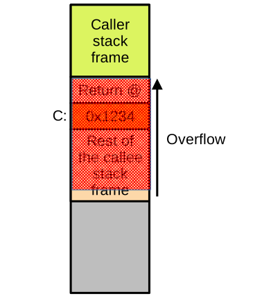
With the canary overwritten, the check when the function returns will fail, detecting the attack.
By default, with modern compilers only certain functions (declaring a char array > 8 bytes) are protected with canaries.
Use -fstack-protector-strong to apply it to more functions (no size limit), and -fstack-protector-all applies it to all functions.
More canaries will increase the security of your program, but will also increase performance and code size overheads: there is a trade-off to make here between security and code size increase/performance impact.
Canaries are not a perfect protection. With current implementations, the same canary value is used to protect all function calls. This means that if the attacker can leak the canary value, for example if there is an overflow in read mode on the stack, then the protection is broken for the entire program.
Other Common Hardening Techniques
Stripping Symbols. Other common protection techniques include stripping your program from symbols and debug information. This makes reverse engineering your code, which is a crucial step in most attacks as we will see in this unit’s lab exercises, much more difficult. To strip a particular binary use:
$ strip <binary>
Read-only Relocations (RELRO). RELRO protects against attacks using the shared library relocation system (Global Offset Table) to hijack a program’s control flow. Relocations represent the resolution of calls to shared libraries at runtime: you can see these as a form of function pointers that an attacker can try to overwrite. Partial and full RELRO sets part or all of the address space areas holding relocation information as read-only. Here we again have a trade-off between security and performance overhead, as full RELRO will significantly increase load time.
RELRO is enabled at the level of the linker. To enable partial RELRO, pass these flags to the compiler (that will itself pass them down to the linker):
$ gcc program.c -Wl,-z,relro -o program
To enable full RELRO:
$ gcc program.c -Wl,-z,relro,-z,now -o program
_FORTIFY_SOURCE macro.
This macro enables some lightweight compile-time/runtime buffer overflow protection checks before sensitive functions such as strcpy, strcat, etc.
It can be enabled through the compiler invocation
$ gcc program.c -D_FORTIFY_SOURCE=1 -o program
A second level is available (-D_FORTIFY_SOURCE=2).
It enables more checks but may break the program.
checksec.
A binary can be analysed to check for the presence or absence of the hardening techniques we covered here, using the checksec tool.
Here is an example of usage:
$ gcc -fstack-protector-strong -D_FORTIFY_SOURCE=2 -O2 -Wl,-z,relro -Wl,-z,now myapp.c -o myapp
$ strip myapp
$ checksec --file myapp
RELRO         STACK CANARY    NX            PIE            Symbols       FORTIFY
Full RELRO    Canary found    NX enabled    PIE enabled    No Symbols    Yes
checksec reports on the presence and status of RELRO, stack canary, NX bit, debug and other strippable symbols, and FORTIFY_SOURCE.
The PIE field here indicates whether the binary is a position independent executable (PIE), a technology that allows loading segments of the binary anywhere in the address space – something required for ASLR.
Control Flow Integrity
Here we cover with a bit more details a last, more advanced, technique, named control flow integrity (CFI). We have seen previously how control flow hijacking attacks such as stack smashing force the program to take illegitimate code paths in the control flow graph, i.e. code paths that were not intended by the programmer when the source code was written. CFI enforces that the code paths executed at runtime by the program conform to the CFG originally intended by the programmer.
CFI generally involves two protections:
- Forward-edge CFI, checking that function pointers and C++ virtual tables always have legitimate targets.
- Backward edge CFI, checking that return addresses also always have legitimate targets.
CFI: Forward Edge Protection. Regarding forward edge protection, CFI enforces that when a function pointer or an entry in a C++ virtual table is called, the target should be a valid function. What valid means here depends on the implementation: with coarse-grained CFI, the protection will just check that the target is the beginning of a function. With fine-grained CFI, the protection will make sure that only the functions whose addresses are assigned to the function pointer or virtual table in the code can be called.
LLVM/Clang has a software implementation of CFI; to enable it, add the following compiler flags:
$ clang -g -fsanitize=cfi -flto -fvisibility=hidden program.c -o program
This will instruct the compiler to insert the necessary instrumentation for CFI checks.
Recent Intel processors also have CFI in hardware through a technology called Intel Control-Flow Enforcement.
A special instruction endbranch64 marks valid targets for indirect branches, such as virtual table member invocations.
CFI: Backward Edge Protection. Regarding backward edge protection, which protects the return address on the stack, this is achieved for CFI with what is called a shadow stack. The shadow stack is a separate stack that stores a copy of the return address upon each function call. When the callee returns, the return address to jump to is checked against the copy in the shadow stack: if they don’t match, it may be indicative of an attack.
Here is an illustration of the shadow stack:
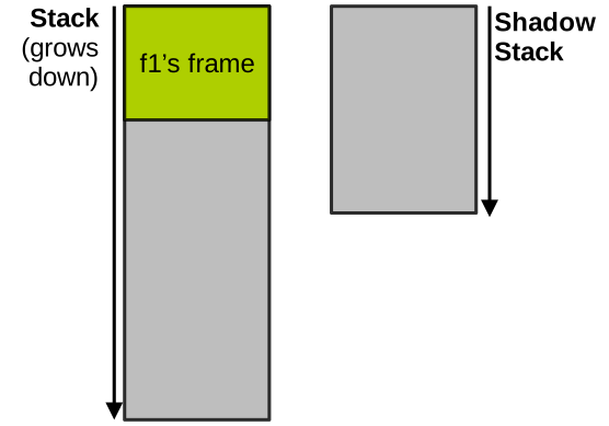
Assume we are running the code of a function f1, we have its frame on the stack, and the shadow stack which is empty for now.
When f1 calls f2, it pushes the return address on the stack normally, but also a copy of it on the shadow stack:
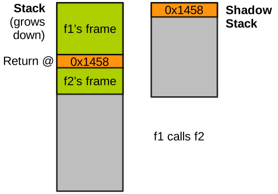
Assume that f2 calls a function f3, which itself calls another function f4.
The process repeats with each function call: the return address is pushed normally on the stack and a copy is placed in the shadow stack.
When f4 runs we have the following:
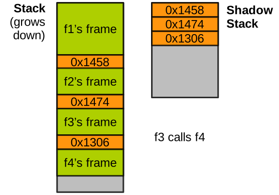
When f4 returns to f3, the return address on the stack is checked against the corresponding entry in the shadow stack; if they match, all is well.
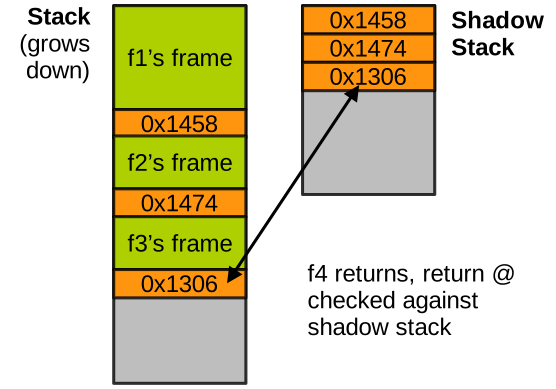
If, during the execution of f4, an overflow lets the attacker overwrite the return address, the check would fail.
After the check, the return address copy is popped from the shadow stack.
As the program returns from f3 to f2 and then from f2 to f1, similar checks are done.
Of course the shadow stack needs to be placed by the compiler at a location in memory that is very hard for an attacker to access. Clang’s implementation randomises that location and protects it with unmapped guard pages that will fault if accessed, however the shadow stack itself needs to stay readable and writable by the program to perform its function. Hardware shadow stack implementations provide stronger protection, and the shadow stack content can generally not be accessed with standard loads and stores, only with specific shadow stack manipulation instructions.
Memory Safety: Further Readings
Memory Errors and Their Exploitation
- Szekeres et al., SoK: Eternal War in Memory. Must read, everything you need to know about memory safety as of 2013.
- Aleph One, Smashing the Stack for Fun and Profit. Seminal paper on the stack smashing attack.
- Akritidis, Cling: A Memory Allocator to Mitigate Dangling Pointers. Good presentation of attacks leveraging use after free (+ propose a solution).
- Shacham, The Geometry of Innocent Flesh on the Bone: Return-into-libc without Function Calls (on the x86). Seminal paper about return oriented programming.
- (Book) Erickson, Hacking: The Art of Exploitation. See chapter 3, “Exploitation”.
Secure Coding in C/C++
- Carnegie Mellon’s Software Engineering Institute, CERT C Coding Standard.
- (Book) Seacord, Secure coding in C and C++.
- ISO/IEC, TS 17961 C Secure Coding Rules.
- NASA JPL, C Coding Standard.
- Fedora’s Defensive Coding Guide.
Detecting Bugs Offline
- Clang static analyser’s website.
- Song et al, SoK: Sanitizing for Security. Everything you need to know about sanitisers.
- Nethercote and Seward, Valgrind: A Framework for Heavyweight Dynamic Binary Instrumentation. Valgrind’s paper.
Runtime Defences
Operating Systems: Introduction
You can access the slides 🖼️ for this lecture.
Here we start to discuss operating systems and the relevant security aspects.
What is an Operating System?
An operating system (OS) is a piece of software that manages hardware and software resources by acting as an intermediary layer between users/applications and the computer’s hardware. The interface exposed by the operating system to users and applications is both convenient to use and secure. Well-known examples of OSes are Windows, Linux, or macOS.
From a very high-level point of view, the intermediary layer that is the operating system on a computer can be represented as follows:
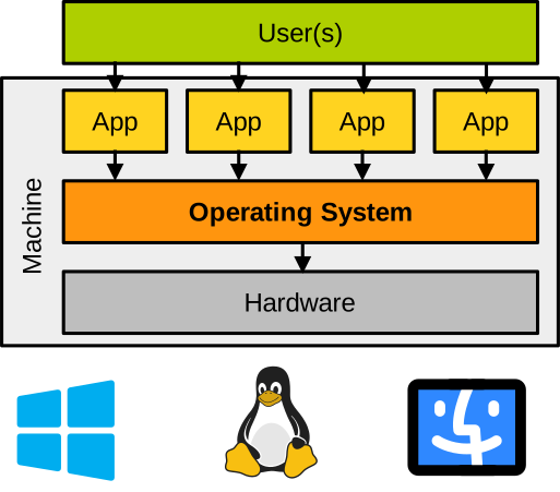
Functions of an Operating System
An operating system provides many functionalities, named services. We can classify some of the most crucial services of an OS based on the type of hardware component they manage:
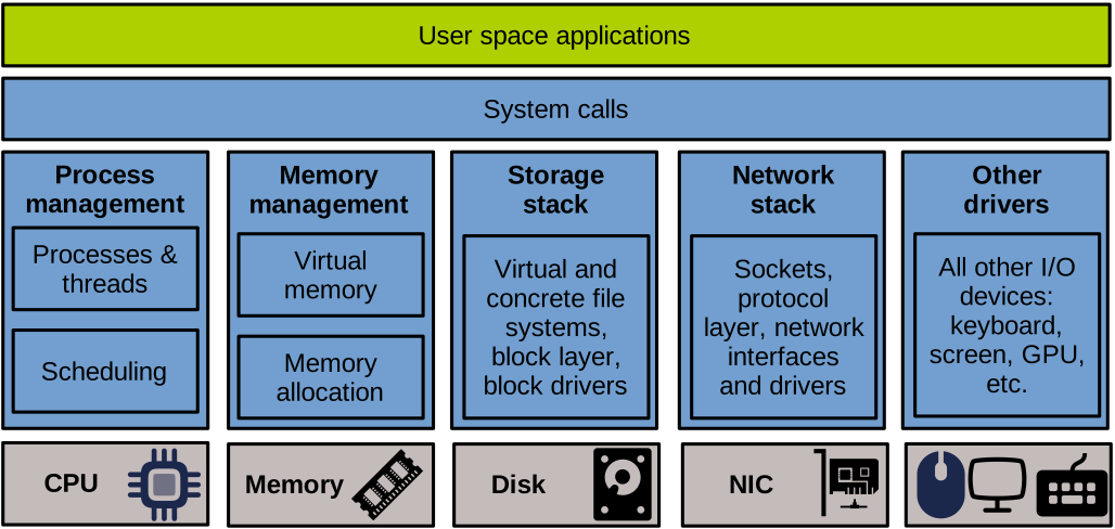
System Calls. The system call layer represents the API exposed by the operating system to applications. It is the one and only interface through which applications can call the OS in order to request services.
CPU Management Services. To let programs execute on the CPU, the operating system creates abstractions such as processes and threads, and offers services to manage these abstractions. These services let applications create and destroy processes and threads, manage their state and life cycle, context switch them in and out of the CPU, let them communicate via inter-process communication mechanisms, and synchronise using locks or notification primitives, allocate resources for their execution, etc. A particular and well-known service relevant to process and thread management is scheduling: it is the component of the OS that decides which process/thread should run on the CPU, and for how long.
Memory Management Services. To let programs use memory, the OS provides services for programs to allocate/deallocate memory. The OS also manages virtual memory to create and maintain programs’ address spaces, enforce memory protection, establish memory sharing between communicating applications, swap pages to disk, etc.
Storage Services. Most OSes implement a storage stack to let applications access secondary storage. Such stacks are generally quite complex and multi-layered, with a virtual file system exposing a common file abstraction to applications, file systems handling file access requests, a block layer abstracting and optimising access to disk-like devices, and device drivers managing particular models of disks.
Network Services. OSes also integrate network stacks that are, similarly to storage stacks, complex and made of multiple software abstraction layers piled on top of each other. The socket layer exposes a practical interface for applications to access the network. Transport layers handle packets of data to send/receive. Network layers take care of packet routing and delivery, and lower-level layers manage MAC addressing and also include network device drivers.
Other Services and Drivers. OSes implement many other services including time management, power management, resource virtualisation (e.g., containers), display and sound management, etc. Beyond storage and networking, OSes also implement other drivers for a plethora of I/O devices such as keyboards and mice, screens, printers, sound devices, GPUs, etc.
A (Very) Brief History of Operating Systems
In the 1950s and 1960s, the ancestors of today’s operating systems were called resident monitors. In essence, they were glorified punch card/magnetic tape queue managers: the resident monitor would execute on a batch system, loading and running programs (jobs) sequentially from a queue, one after the other. The term resident denotes the fact that, unlike programs, the monitor would always be present in memory to clean up after a program’s execution and load the next one. An example of a resident monitor from 1960 is IBSYS, running on IBM’s mainframe computers.
In the 1970s, time-sharing systems appeared: several users and several programs could use the same computer at the same time. The sharing of the computer brought relevant security issues: how to isolate users and programs to avoid disturbances or attacks? Unix (Bell Labs) is a prime example of such time-sharing systems. The Unix OS kernel was originally written in (architecture-specific) assembly in 1970, and the C programming language was developed to build cross-architecture programs aimed at running on top of Unix. The Unix kernel ended up being mostly re-implemented in C to make it portable across architectures. This is one of the machines Unix was running on, a DEC PDP 11:
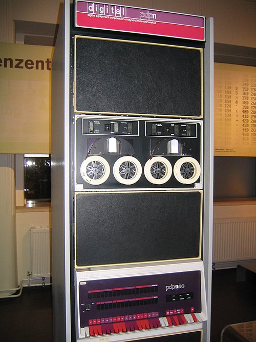
Personal computers became popular in the 1980s. Their first OSes ran on the command line only, e.g., Microsoft’s MS-DOS, then GUI-based OSes appeared in the 1990s-2000s. The main ones are still very active today, although they have evolved considerably since their inception: Windows, Linux, or macOS. The 2000s saw the rise of networking and Internet support, which raised security requirements as computers networked together may not trust each other. Personal computer OSes also quickly saw an explosion of the software (applications, libraries) and hardware (CPU architectures, devices) they needed to support, earning them the label of general-purpose operating systems.
In the 2010s, we have seen the explosion of mobile computing and associated OSes (Android, iOS). Another technology that took off is cloud computing, which was made possible by a series of OS technologies, notably virtualisation (virtual machines, containers), enabling several operating systems to run on the same machine. In both mobile and cloud computing, security aspects are absolutely critical: modern smartphones may contain tons of personal data, and, as we will see in the virtualisation part of this unit, the entire business model of cloud computing rests on the trust that the tenants sharing a physical machine are properly isolated from each other.
In contrast to general-purpose OSes, many specialised OSes have been proposed, focusing on particular types of hardware and/or applications in order to optimise various performance objectives such as computation speed, memory footprint, reliability, power consumption, etc. An important class of specialised operating systems, embedded and real-time OSes, began in the 1980s with the rise of microcontrollers. They cater for very specific constraints such as the limited amount of resources (RAM/CPU power) of these platforms, power consumption requirements, the need to complete certain operations in bounded time, etc. Embedded and real-time OSes are still very relevant today (e.g., IoT/Edge computing) and security/safety is a central concept in most usage scenarios.
OS Architectures
OSes can be classified based on their internal software architecture, i.e., how the different components (services) making up an OS kernel are organised together. That aspect of OS design has a significant impact on their performance and security guarantees.
The monolithic kernel OS model (e.g., Linux) packs all OS services tightly together to maximise performance. There is no isolation between services, which raises security concerns. The microkernel OS model (e.g., Minix, QNX) establishes a minimal kernel, the microkernel itself, with core services (scheduling, memory management, etc.) running with full privileges on the machine, decoupled from other services (filesystem, device drivers, etc.) that are isolated from each other and from the microkernel. This yields security benefits at the cost of a performance slowdown compared to monolithic solutions. More exotic/research OS models have been proposed, generally consisting of various forms of specialised OSes: multikernel, exokernel, unikernel, etc. We will discuss the security implications of monolithic, microkernel, and other modern OS models later in the unit.
OS Kernel vs. Distribution
An important terminology distinction to make at this stage of the unit is the difference between an OS kernel and an OS distribution. An OS kernel represents the code and data for the program that is the operating system: on a standard machine, it is the only piece of software that can control the hardware directly. Examples of OS kernels include Linux, the Windows NT kernel, the macOS XNU kernel, etc. An OS distribution is a set of software that includes a kernel and a series of additional programs representing system utilities: libraries, package managers, a graphical user interface, some default applications, etc. Examples of OS distributions include Ubuntu, Fedora (both Linux-based), Windows 11, macOS, etc.
The difference between a kernel and a distribution can be illustrated as follows:
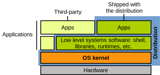
⚠️ OS distributions are sometimes referred to as “operating systems”, although they contain much more than the OS, and many of the applications/libraries they embed have little to do with the goals and objectives of an OS. In this course unit, when we mention an operating system we refer to an OS kernel, not an OS distribution.
Security Aspects
Security Goals of an OS. An OS aims to provide convenient resource mechanisms for applications: processes, filesystems, memory management, etc. For performance reasons, the OS must efficiently multiplex (schedule) the accesses by applications to the resources in question. Moreover, the OS is also in total control of the machine and, as such, is in charge of ensuring the security of all applications.
Here, security implies the correct design and implementation of the OS’s resource management and scheduling strategies. Depending on its trust model, a secure OS must not allow an application to access the address space of another application, to write to a file it does not have permission to access, or to hog the CPU at the expense of other applications. In practice, such issues can happen when OS mechanisms are misused inadvertently (fault tolerance), and, most importantly, maliciously (adversarial context). In absolute terms, the concept of a secure operating system is an oxymoron, an ideal goal that can hardly be fully achieved, as no system of modern complexity is entirely secure.
The security goals stated by an OS generally describe which subjects (e.g., applications, users) can or cannot perform what operations (e.g., read, write, execute) on what objects (e.g., files, sockets, bytes in memory). With these goals in mind, the OS aims to apply the principle of least privilege and maintain confidentiality/integrity/availability. Being as secure as possible means approaching as much as possible a state of least-privilege, and that objective is often at odds with other goals of OSes, namely performance and convenience of usage.
OS Trust Models. The trusted computing base (TCB) of an OS is the set of components enforcing security goals. The OS TCB needs to:
- Mediate all security-sensitive operations.
- Be correct.
- Not be tampered with by software outside the TCB.
An OS’s TCB depends on the security objectives and the application scenario, but generally includes the hardware, boot process, all OS code, and some privileged applications:
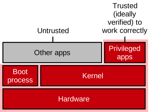
That is a huge amount of software and hardware that we trust to run the computers we are increasingly reliant upon! An OS’s TCB can be hard to precisely define, and it is generally impossible to formally prove its correctness.
Threat Models.
A threat model defines what an attacker can do. For an OS, the threat model generally encompasses a plethora of attacks coming from a variety of vectors. Examples include:
- A remote attacker sending malformed network packets.
- A local attacker using a malicious user application, trying to escalate privilege and become root.
- A malicious hardware device misbehaving, trying to compromise the driver/OS code.
- A compromised boot process loading malicious kernel components or a rootkit.
- An attacker accessing the kernel log to steal sensitive information (e.g. to break certain defences such as ASLR) or to erase traces of intrusion.
- Etc.
Operating Systems: Basic Practical Aspects
You can access the slides 🖼️ for this lecture.
In this part of the unit we present an extremely simplified model of how an OS runs on an extremely simplified model of modern computer hardware. In doing so, we investigate what the OS expects from the hardware, what security properties an OS needs to enforce, and how it does so. Concerning the hardware, we focus on CPU and memory. We will see how the OS interfaces with devices (I/O) later.
Basic OS Principles
A computer is made of hardware: CPU, memory, and I/O (disk and network). Software runs on top of that hardware, and the OS manipulates the hardware directly: in most scenarios the OS is the lowest layer of software in direct contact with the hardware. Applications represent higher-level layers: they run on top of the OS. In other words, applications need to go through the OS to do anything important with the hardware:
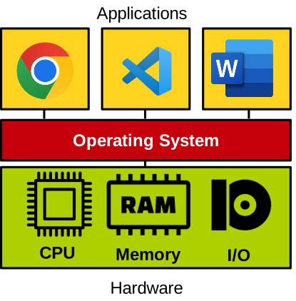
This is mandatory for safety and security reasons, as we cannot let applications access the hardware without the supervision of the OS. Letting applications manipulate the hardware directly would lead to problems such as a malicious application accessing the memory of another application, or a faulty application crashing the entire computer.
The OS provides standardised abstractions for applications to use the hardware safely: processes and threads for CPU/memory, filesystem for storage, sockets for network, etc. These abstractions are accessed through a standard API, system calls (sometimes abbreviated syscalls):
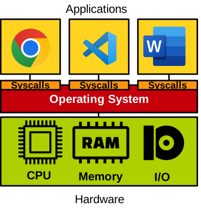
On Linux, examples of system calls are open, read, write, mmap, etc.
You can see the full list of system calls supported by Linux here.
Boot Time
Below is a simplified illustration of what runs on a CPU when a computer starts:

The basic steps are:
- Power on.
- The motherboard firmware (BIOS) runs first, and performs basic hardware initialisation.
- The BIOS loads the bootloader (e.g., GRUB), which begins to run.
- The OS kernel is loaded by the bootloader, and begins to run.
- The OS boots: it initialises more hardware as well as itself.
- Once the OS’ initialisation is done (dashed line), it can run applications.
For the sake of simplicity, we assume a single core here, i.e., only a single program can run at a time. Here we use the term program in a broad sense: it can be an application, the OS kernel, the bootloader, etc. Once the OS finishes booting (dashed line above), the CPU mostly runs applications. These applications are, from time to time, interrupted to execute the operating system.
Execution Model on the CPU
A basic CPU contains, among other things, an Arithmetic Logic Unit (ALU), some control logic, and registers. One particular register is the instruction pointer (or program counter): it points within the code segment to the instruction currently being executed by the CPU. General-purpose registers are used to hold the operands for operations realised in the ALU. Data can be loaded from memory into registers with load instructions, and stored from registers into memory with store instructions.
For now let’s just assume that our CPU accesses physical memory directly without any form of virtual memory. With that in mind, an application App 1 running on the CPU can be illustrated as follows:
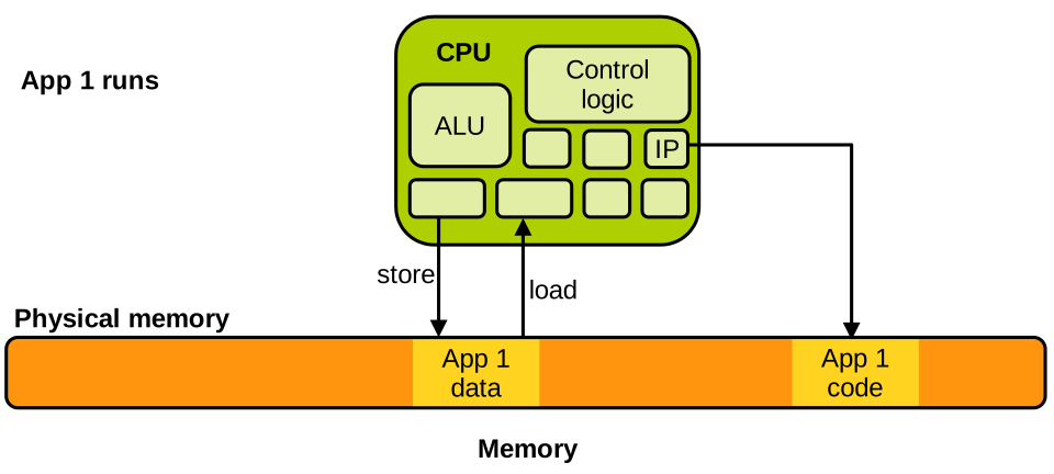
When another application App 2 runs, we have something similar:
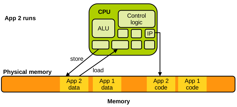
Obviously, App 2’s data and code segments are present at different locations compared to App 1’s. The OS kernel is no different: it also has data and code segments, and when it runs on the CPU we have:
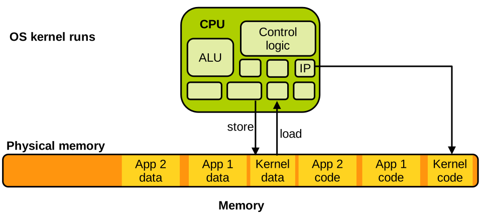
The state of an application at any given point in time during its execution on the CPU corresponds to the content of the CPU registers. It can be easily saved and restored to/from RAM. One scenario in which this is needed is a context switch. Assume that App 1 is running on the CPU, but the scheduler decides that App 2 should run instead: App 1 needs to be removed from the CPU and replaced by App 2. This is a two-step process, illustrated below:
- Saving App 1’s CPU execution state in memory (step A below). That state is, once again, the content of CPU registers.
- Loading App 2‘s CPU execution state (registers’ content) from memory into the CPU (step C below). That loaded state has been either saved in memory the last time App 2 was context-switched out of the CPU, or it is an initialisation state if App 2 has just started to execute.
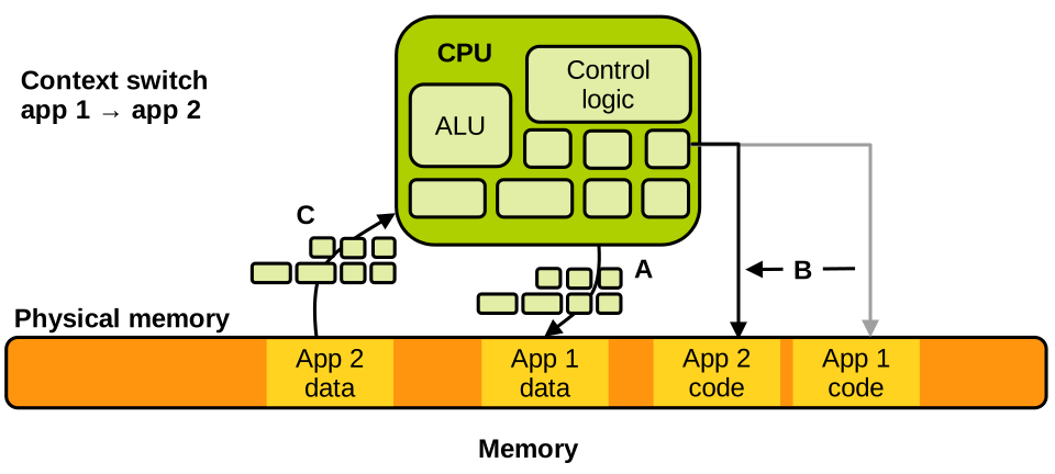
Once the state for App 2 has been loaded, the instruction pointer register will point to whatever instruction App 2 was executing the last time it was context-switched out of the CPU, or to its entry point if it just started running. The context switch is done, and the execution of App 2 can then resume.
From a high-level point of view, context switches work as described with all modern CPUs. The key idea is that being context-switched in and out of the CPU is completely transparent from the applications’ point of view: their code is not aware of (and does not need to manage) the fact that their execution may be interrupted/restored at any time.
Kernel Invocation
We have seen that our CPU alternatively executes kernel and application code. Application code runs when applications are context-switched on the CPU. What about the kernel? When does the CPU start executing kernel code? Kernel code runs on the CPU only on 2 types of occasions:
- At boot time, after the bootloader finishes loading the kernel, as we have seen (step 5 in our boot time model above); and
- At runtime, when an interrupt is received by the processor.
That’s it: past boot time, an interrupt is the only way for the CPU to enter the kernel and start to run OS code. There are 2 types of interrupts:
- Hardware interrupts. These are notifications from I/O devices; for example, a network card sends an interrupt to the CPU to notify it that a network packet has arrived.
- Software exceptions. These are instances of the CPU interrupting itself; for example, because it executed an incorrect operation such as a division by zero.
Let’s see what happens on the CPU when an interrupt is received. Assume the CPU is running App 1:
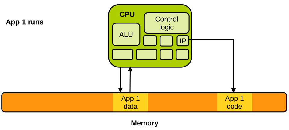
Now assume the CPU receives a hardware interrupt from an I/O device. As soon as the interrupt is received, the CPU pauses the execution of App 1 and saves its execution state (CPU registers) in memory, similarly to what we have seen with a context switch. Next, a predefined kernel execution state is loaded on the CPU:
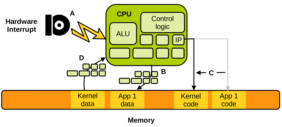
That predefined OS execution state corresponds to the entry point of the hardware interrupt handler, i.e., the code responsible for determining what to do when a hardware interrupt is received. That code will determine what hardware interrupt has been received and act accordingly. For example, in the case of a received network packet, it will acknowledge the interrupt and schedule the packet to be retrieved from the network card. Once the interrupt handler is done, the kernel stops running and the state of the previously interrupted application App 1 is restored:
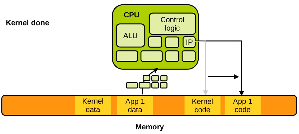
Similar to the context switch we saw earlier, the interrupt handling by the OS is completely transparent from the applications’ point of view. In the case of a software exception, for example if App 1 runs and its code executes a division by zero, things work exactly the same. App 1 is interrupted, its state is saved in memory, and the kernel starts to run:
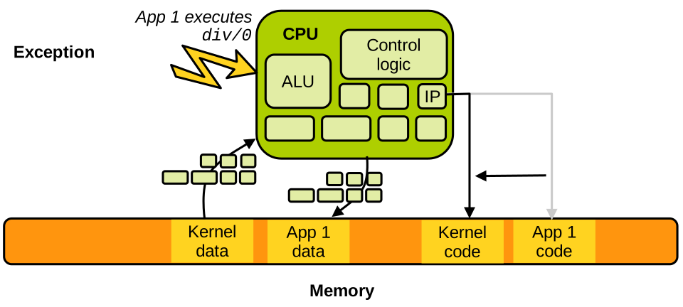
The kernel state that will be loaded here is the entry point for the division by zero interrupt handler. Once the handler is done, the kernel resumes the execution of the application. Note that upon an unrecoverable exception, which is generally the case for a division by zero, the kernel will kill the application and resume the execution of another application. Other exceptions are recoverable, for example a page fault triggering on-demand memory allocation.
OS Security Principles
A crucial OS security invariant is that we cannot have an application read/write the memory of another application or of the kernel. If that invariant is not maintained at all times, there can be no security guarantees in our system. An application reading/writing the memory of another application may be stealing passwords/secrets, or tampering with critical data and code. An application reading/writing the memory of the kernel could achieve the same objectives, as the kernel is a privileged component that can generally access all the memory in the system. So we absolutely want to avoid this happening:
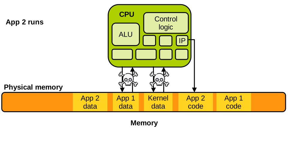
To enforce that invariant, the OS sets up the CPU’s MMU to enable virtual memory and perform virtual-to-physical address mapping. With virtual memory, an application is tricked into thinking it has access to 100% of the memory: its virtual address space. The address space of each application is set up in such a way that it does not contain any memory that the application is not supposed to address. For example App 1’s virtual address space contains only its code and data:
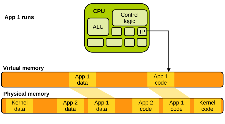
The same applies to App 2:
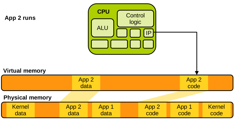
The kernel generally needs to access the entirety of memory:
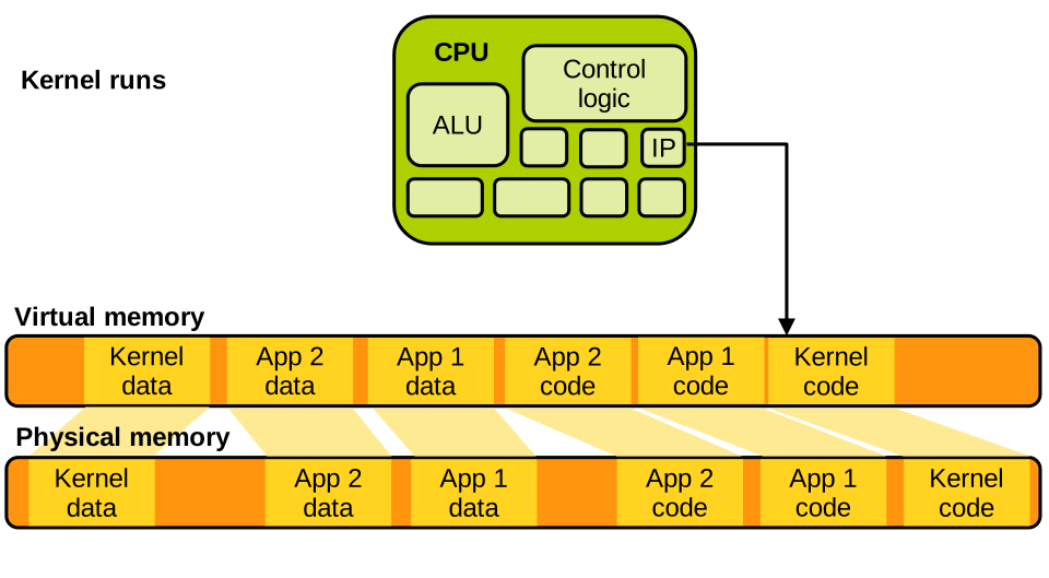
The address space of an application does not map the physical memory relating to other applications or to the kernel: this way, the key security invariant mentioned above is enforced.
System Calls
Based on what we just discussed, if an application cannot access kernel data/run kernel code for security reasons, how can it invoke OS services?
As we know, the only way for an application to call the OS is to issue a system call. It works as follows: when invoking a system call, the application executes a special instruction that triggers an exception; as with other interrupts and exceptions, the CPU interrupts the application and starts running the kernel to manage the system call:
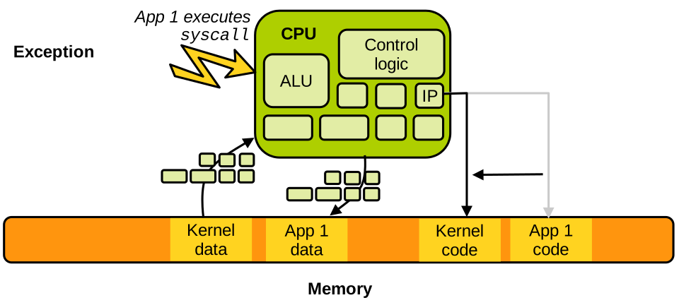
Application programmers generally do not invoke system calls directly, but rather do so through the use of libraries.
Many functions exposed by the C standard library, such as read(), write(), etc., have a similar name and prototype as the system call they invoke, providing a language/source-level interface to the OS.
That source-level interface is called an Application Programming Interface (API): a source-level communication interface and convention for software components tightly coupled (e.g., compiled) together.
The libc itself often needs to invoke the OS to issue system calls. We cannot rely on an API to achieve that, because the libc and the kernel are two software components that are not compiled together. More generally, the kernel cannot assume that applications/libraries invoking it are written in any particular programming language, so we need a communication interface and convention operating at the binary level, an Application Binary Interface (ABI). This machine-level convention defines how to invoke a system call on a particular architecture:
- What parameters to put in what registers upon invocation.
- What machine instruction(s) to use to effectively trigger the exception to switch to the OS.
- What register should hold the return value when returning from the OS.
Linux uses the System V ABI, which states that for x86-64 a system call is invoked by an application as follows.
- Place arguments in order in the
%rdi,%rsi,%rdx,%r10,%r8and%r9registers. - Place the system call identifier, which is an integer identifying uniquely what system call to invoke, in the
%raxregister. - Invoke the
syscallinstruction, which triggers the exception and traps to the kernel. - Upon return to user space, the kernel places the system call return value in
%rax.
To see an example of this ABI in action, let’s take a look at the disassembled Libc function clock_gettime, that invokes the system call of the same name:
00000000004672b0 <__clock_gettime>:
#...
  4672f8:	mov    %r12,%rsi
  4672fb:	mov    %ebp,%edi
  4672fd:	mov    $0xe4,%eax
* 467302:	syscall
# ...
As we can see, the first parameter, the integer clk_id, is first placed in %rsi (moved from another register).
Then the second parameter is set up in %rdi in the same way (recall that %edi are the lower 32 bits of %rdi).
Finally, the system call identifier of clock_gettime is placed in %rax: it is 0xe4, which is 228 in base 10. You can confirm that it corresponds to clock_gettime in the Linux system call table.
At that stage the system call is ready to be invoked: executing the syscall instruction will trigger an exception and switch to the OS, which will inspect the content of the registers to determine what system call is being invoked, with what parameters, and act accordingly.
Invoking a System Call Manually.
Now that we know how a system call is invoked by an application/library, we can try to invoke one manually by exercising the ABI with a bit of assembly code.
Below is an assembly program that prints "Hello, world!" to the standard output.
This can be realised by calling a single system call, write, on the file descriptor corresponding to the standard output (1).
.global _start

.text
_start:
    # write(1, message, 14)
    mov $1, %rax
    mov $1, %rdi
    mov $message, %rsi
    mov $14, %rdx
    syscall

    # exit(0)
    mov $60, %rax
    xor %rdi, %rdi
    syscall

message:
    .ascii "Hello, world!\n"
This program first prepares the invocation of the write system call: it places the write system call identifier (1) in %rax.
Then it places the first parameter 1 (standard output’s file descriptor) in %rdi, the second parameter (a pointer to "Hello, world!\n") in %rsi, and the number of characters to write (14) in %rdx.
write is then invoked with a syscall instruction, which should produce the output.
Once that is done, we can exit the program with an exit(0) system call: we place exit’s identifier (60) in %rax, 0 in %rdi (xor’ing a register with itself is a fast way to zero its content), and we execute syscall.
The program can be assembled, linked, and executed as follows:
$ as syscall.s -o syscall.o
$ ld syscall.o -o syscall
$ ./syscall
Hello, world!
Privilege Modes
Some CPU instructions are privileged, and they should only be executed by the kernel. Examples include the instructions that allow installing new page tables, communicating with I/O devices, shutting down/resetting the CPU, etc. If applications could run these instructions freely without supervision from the OS, all the security guarantees that an OS is trying to enforce would break. To make sure only the OS (and not applications) can invoke these instructions, modern CPUs implement privilege modes. At any time the processor can be in one of two modes:
- User mode, when applications run.
- Supervisor mode (also known as kernel mode), when the kernel runs.
When a privileged instruction is executed, it succeeds if the CPU is in kernel mode, and triggers an exception, trapping to the kernel, if executed in user mode. This way, any attempt by applications to invoke privileged instructions can be caught by the OS and mediated/prevented based on the situation.
Privilege modes have various names according to the architecture; on x86 they are called protection rings. For x86-32, we have the following:
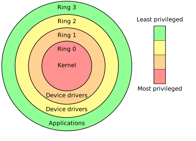
Ring 0 represents the highest privilege level: this is where the OS kernel executes, and all instructions can be freely invoked in that ring. Ring 3 is the lowest privilege level, restricting the use of all privileged instructions: this is where the applications run. Rings 1 and 2 represented intermediate privilege levels on x86-32, and were used to run deprivileged kernel components such as drivers. These were dropped in x86-64, leaving only ring 0 (supervisor mode, for the kernel) and ring 3 (user mode, for applications).
User/Kernel World Switches.
On x86-64, when the syscall instruction is invoked, the CPU switches from user mode (running the application) to supervisor mode (running the kernel).
It then jumps to a predefined piece of code, the system call handler.
This is a form of control flow integrity: any system call invoked by the application will run the same kernel system call handler, which performs all the necessary checks on the system call parameters.
The kernel starts to run and handles the syscall.
Once done, the kernel executes the sysret instruction, which triggers the return to user code by switching the CPU to user mode and jumping to the instruction following the syscall in the application code.
That process can be illustrated as follows:

Switches in both directions between user and kernel mode are called world switches. From the performance point of view, such world switches are very costly: they take hundreds, if not thousands of CPU cycles, among other overheads such as cache pollution.
Process Management
You can access the slides 🖼️ for this lecture.
Here we discuss one of the core responsibilities of an operating system: process management. As mentioned previously, we will focus on Linux.
Processes
A process is an instance of a running program in the system. The OS gives each program the illusion that it runs alone and has exclusive access to all of the machine’s resources. This way, all applications in the system can run independently of each other. This is achieved as follows:
-
Regarding memory, each process has its own address space, and it can address most of it.
-
Regarding the CPU, each process is scheduled in and out of the CPU completely transparently.
-
A process also has handles to system resources maintained by the kernel: file descriptors, sockets, etc., and an execution state/context: the values in CPU registers at any given point in the program’s execution.
Process Identifiers (PIDs).
Each process has a unique integer identifier in the system, called the process identifier, the PID.
A process can obtain its PID with the getpid system call.
Below is an example of a C program printing its PID to standard output:
#include <stdio.h>
#include <stdlib.h>
#include <unistd.h>

int main() {
    printf("my pid is: %d\n", getpid());
    return 0;
}
We can list all processes running in the system with their pid with the following command:
$ ps -e
The Process Tree.
Apart from the first process created from scratch right after the kernel boots, every other process is created by another process: a parent/child relationship therefore exists between the creating process, the parent, and the created process, the child.
After the kernel boots it creates the first process which gets the PID 1.
This process has historically been called init, but can take different names.
PID 1 then creates children, that may create children, etc.
As such all processes in the system can be represented in a process tree.
The process tree illustrating the parent/child relationships of all processes in the system can be obtained with the pstree command:
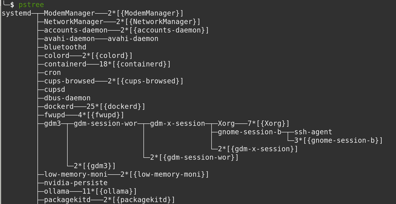
Process Creation with fork()
The only way to create a process in a POSIX-like operating system such as Linux is through the fork() primitive.
It dates back to the 1960s and is now part of the POSIX operating system interface standard.
When a parent process calls fork, it creates a child process.
The child is not created empty: it is actually a duplicate of the parent: it inherits a copy of the parent address space (including all the program’s code and data), system resources such as file descriptors, and even a copy of the parent’s CPU registers’ content at the time fork was called.
With Linux, under the hood fork is implemented by the C standard library that calls the clone system call, which in turn performs the child creation and duplicates the parent’s resources.
After fork is called by a parent process, both the parent and the child return from that call (recall that the child inherits the same code as the parent).
At that stage both processes run concurrently.
This is illustrated in the diagram below, showing a parent with PID 42 that calls fork a first time and creates a child with PID 43.
The original parent then calls fork a second time and creates another child, PID 46:
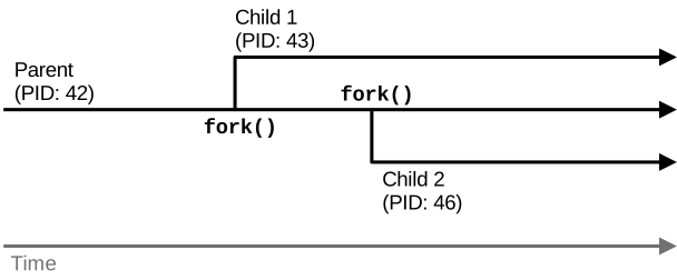
An example of usage of fork is shown below:
int global = 42;

int main() {
  int local = 10;
  printf("[%d] parent before update local = %d, global = %d\n", getpid(),
      local, global);

  int pid = fork();
  switch(pid) {
    case -1:
      printf("fork error!\n");
      return -1;

    case 0: // Child run
      printf("[%d] child, before update local = %d, global = %d\n", getpid(),
          local, global);
      local = 100; global = 100;
      printf("[%d] child after update local = %d, global = %d\n", getpid(),
          local, global);
      break;

    default: // Parent run
      local = 0;  global = 0;
      printf("[%d] parent after update local = %d, global = %d\n", getpid(),
          local, global);
  }

  return 0; // executed by both
}
Our program starts by printing the values of a local variable and a global one, then calls fork and switches on its return value:
- If
forkreturns -1, there was a problem with the call and no child was created: we simply exit the program. - If
forkreturns 0, this means we are in the return path of the child. We print the values of the variables, then set both to 100 and print them again. - If
forkreturns something other than -1 or 0, this means we are in the return path of the parent. Here the parent sets both variables to 0 and prints them.
Then both processes leave the switch body and exit by returning 0 from their main function.
An example of execution of this program is as follows:
$ gcc fork.c -o fork
$ ./fork
[14434] I'm the parent, before I modify them local = 10, global = 42
[14434] I'm the parent, after I modify them local = 0, global = 0
[14434] bye!
[14435] I'm the child, before I modify them local = 10, global = 42
[14435] I'm the child, after I modify them local = 100, global = 100
[14435] bye!
We can see that the child sees the same values for the variable before it updates them.
Once the variables are updated, each process has its own copy of their values: this demonstrates that the address space of the child that starts right after fork is a copy of that of the parent, but also that each process has its own private address space, and it is free to read and write to it independently of other processes.
fork Implementation by the OS.
How does the OS duplicate the address space?
It is not a synchronous copy performed at fork time: the parent’s address space contains megabytes, possibly gigabytes, of mapped memory, so copying it all would take too much time and memory space.
The copy is actually realised later, on-demand, when the memory is accessed.
The key idea here is that as long as neither the parent nor the child modify the content of a particular memory page, they can share it: the virtual memory page in the address space of both processes can be mapped in a read-only manner to the same physical page.
Only when the parent or the child actually write to the memory in question will the page be duplicated: that process is called copy-on-write (CoW).
On-demand CoW address space duplication after fork can be illustrated as follows:
When fork returns, the child receives a copy of the parent’s page table: the address spaces are identical, and the mapped virtual pages point to the same physical pages.
Read accesses are performed normally: as long as neither the parent nor the child modifies the memory, neither needs to see different content:
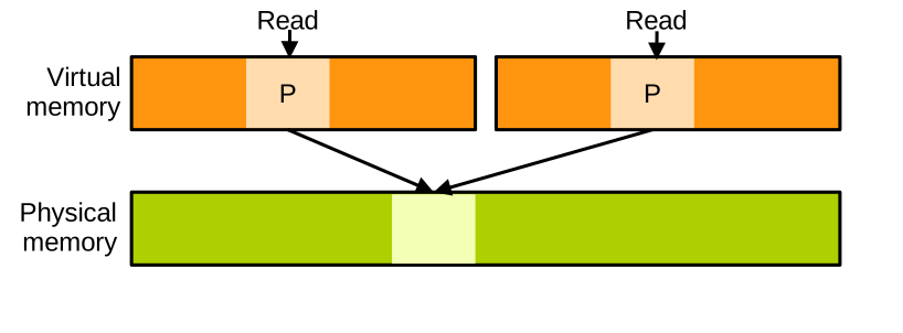
Only when the parent or the child writes to the address space are the corresponding physical memory copied and the page table updated. This is achieved at the granularity of a page, which in the vast majority of systems is 4 KB:
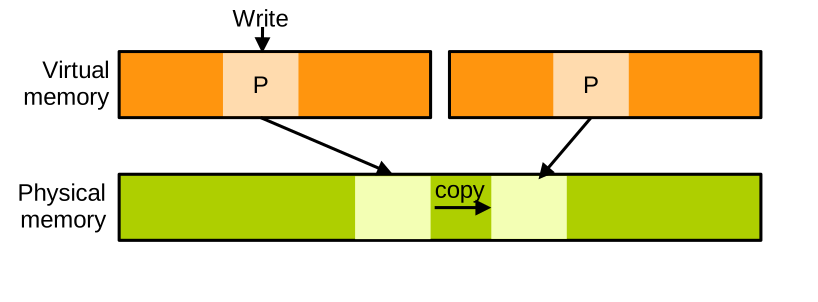
Executing a Different Program with execve
Now what if we want to create a new process to execute a different program, rather than a copy of the parent.
For that we need to combine fork with another primitive: fork + execve.
An example is shown below:
int main() {
    char *args[] = {"/bin/ls", "-l", NULL};
    char *envp[] = {NULL};
    printf("[%d] Parent, forking\n", getpid());

    switch(fork()) {
        case -1:
            printf("fork error!\n");
            return -1;

        case 0:
            printf("[%d] child, calling execve()\n", getpid());
            execve("/bin/ls", args, envp);
            printf("execve error!\n"); // should not reach here
            break;

        default:
            break;
    }
    return 0;
}
In this program the parent calls fork, and the child, in its return path, calls execve.
execve takes as first parameter the path to the binary of the new program we want to execute (here "/bin/ls"), followed by an array of strings, one for each argument (the first being the name of the binary).
The third parameter is the set of environment variables, here just NULL.
If we run this program, we can see that the child executes ls -l successfully:
$ gcc forkexec.c -o forkexec
$ ./forkexec
[19605] Parent, forking
[19606] child, calling execve()
total 60
-rw-r--r-- 1 pierre pierre   931 Jun 19 15:42 fork.c
-rwxr-xr-x 1 pierre pierre 16232 Jun 19 16:32 forkexec
-rw-r--r-- 1 pierre pierre   581 Jun 19 15:42 forkexec.c
-rw-r--r-- 1 pierre pierre  1977 Jun 19 15:42 lock.c
# ...
execve Implementation by the OS.
Under the hood, when a process calls execve, the OS sets up a new blank address space for it.
Whatever was present in the old address space is completely lost.
The kernel has a loader that extracts from the ELF binary to execute the segments that should be loaded, the program entry point, and further metadata indicating whether a user space loader or interpreter is needed:
- If the program to load is a statically-linked binary, it is then loaded directly into the address space.
- Instead, if it is a dynamically-linked binary, or an interpreted script, the kernel will rather load a user space loader or interpreter, with the program/script to execute passed as parameter.
Next, the OS allocates a stack and populates it with what the program needs to initialise: the command line parameters and the environment variables, among other things. Then the OS returns to user space at the program/user space loader/interpreter entry point and starts to execute it. A statically-linked binary will start running directly, a dynamically-linked binary will be loaded and executed by the user space loader, and an interpreted script will be handled by the interpreter.
Inter-Process Communication
Many applications, like web browsers or GUI software, are made of multiple processes working together. This is achieved to leverage parallelism, run background tasks, isolate untrusted code, etc. These processes need to communicate and synchronise:
- Communication between processes is done through Inter-Process Communication (IPC) mechanisms such as pipes, signals, sockets, shared memory, etc.
- Synchronisation lets processes coordinate, so the program does not break when they access memory or other shared resources concurrently. We do not want two processes updating a shared data structure without agreeing on an order of operations, otherwise the data structure may be left in an inconsistent state. Synchronisation is needed, and it is done with mechanisms such as barriers, locks, or processes waiting for each other.
All of these communication and synchronisation mechanisms are provided by the operating system, and most of them are accessed through system calls. Here we cover a few examples of IPC mechanisms first, and then we will discuss synchronisation.
Signals
A signal is a notification sent by the kernel to a process upon certain events, e.g., when the program encounters a page fault or tries to divide by zero, or when the user presses certain combinations of keys (ctrl+c), etc.
A process can also instruct the kernel to send a signal to another process with the kill system call.
In essence, a signal is just a notification: apart from its type (an integer ID), a signal does not carry any data.
A process installs handlers for the signals it wishes to receive and act upon. A process receiving a signal for which it has no handler installed will be terminated by the OS. That is what happens by default upon a segmentation fault or a division by zero.
We can study an example of a process installing a signal handler:
// Signal handler for SIGUSR1
void handle_sigusr1(int signum) {
    printf("[%d] signal received!\n", getpid());
    fflush(stdout); // Ensure immediate output
}

int main() {
    // Install custom handler for SIGUSR1
    struct sigaction sa;
    sa.sa_handler = handle_sigusr1;
    sigemptyset(&sa.sa_mask);   // No additional signals blocked in handler
    sa.sa_flags = SA_RESTART;   // Restart interrupted syscalls automatically

    if (sigaction(SIGUSR1, &sa, NULL) == -1) {
        perror("sigaction");
        exit(EXIT_FAILURE);
    }

    while (1) {
        printf("[%d] Doing useful work\n", getpid());
        sleep(1);  // Simulate work
    }

    return 0;
}
This program first prepares a struct sigaction object, which is a data structure describing a signal handler.
Notice how the sa_handler field specifies the function that will be executed when the signal is received: handle_sigusr1.
The struct sigaction object is then installed with the sigaction system call, in order to handle the signal of type SIGUSR1.
From that point onwards, if the program receives the signal SIGUSR1, the handler handle_sigusr1 will run:
$ gcc signal.c -o signal
$ ./signal
[23800] Doing useful work
[23800] Doing useful work
[23800] Doing useful work
The signal can be sent from another terminal while the main program is running:
$ kill -SIGUSR1 23800
To terminate the program, you can press ctrl+c, which sends a SIGINT signal: our program does not have a handler for it, so it will be terminated by the OS.
Signals: Implementation by the OS.
Under the hood, the kernel delivers signals lazily: upon returning to user space in a process from an interrupt or a system call, the kernel checks if that process has any pending signals.
If so it determines the action: either invoke the handler or terminate the process if there is no handler.
If a handler needs to run, the kernel modifies the execution of the process as follows.
It sets the instruction pointer to return to be the handler’s code, and puts on the stack information about the signal received and what to do when the handler finishes running.
Execution then returns to user space and the handler executes.
When the handler is done, the program invokes the sigreturn system call that will clean things up and resume the normal process execution.
You will notice that the handler in our previous example does not invoke sigreturn directly: this is actually called under the hood by the C standard library when the code of our handler returns.
All these steps are illustrated here:
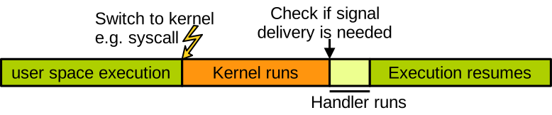
We have a process running in user space. At some point it traps to the kernel, following a system call or an interrupt. After the kernel is done processing this trap, it checks, before returning to user space, if a signal needs to be delivered. If so, it returns to user space at the level of the handler, which runs, and when the handler is done the process resumes its execution normally.
Pipes and Sockets
Contrary to signals, which do not carry much information, pipes and sockets are data communication channels. Pipes are unidirectional: there is one writer process and one reader process, while sockets are bidirectional. Both mechanisms are visible to processes as pseudo files on the filesystem. This is because the filesystem is visible from all processes, so it is easy to share a pipe or a socket between different processes in this way. The kernel uses internal buffers to hold the data in transit on pipes and sockets. The kernel also puts reading and writing processes to sleep when the communication channels are empty or full.
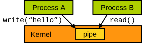
Here is an example of usage of a pipe, also named FIFO:
#define FIFO_PATH "/tmp/myfifo"

int main() {
    mkfifo(FIFO_PATH, 0666); // Create a named pipe (FIFO)

    pid_t pid = fork();
    if (pid == 0) { // --- Child Process: Writer ---
        int fd = open(FIFO_PATH, O_WRONLY);

        const char *msg = "Hello from child!\n";
        write(fd, msg, strlen(msg));
        close(fd);

    } else { // --- Parent Process: Reader ---
        int fd = open(FIFO_PATH, O_RDONLY);

        char buffer[128];

        int n = read(fd, buffer, sizeof(buffer)-1);
        if (n > 0) {
            buffer[n] = '\0';  // Null-terminate
            printf("Parent received: %s", buffer);
        }

        close(fd);
        unlink(FIFO_PATH);  // Clean up FIFO file
    }
}
We have a parent process that creates the pipe with the mkfifo system call.
It then forks to create a child.
The child opens the pipe in write mode and writes a message into it.
Concurrently, the parent opens the pipe in read mode, reads from it, and displays what it read.
Both processes close the pipe’s file descriptor when they are done, and the parent deletes the pipe at the end with the unlink system call.
Shared Memory
The IPC examples we saw all involve quite a lot of system calls, both to be set up and to achieve communication. This is not ideal in terms of performance, as system calls are costly because each user/kernel switch takes many CPU cycles. Further, because the kernel needs to be involved in each data transfer, the data in question needs to be copied as part of the transfer. This is done for security reasons: as we will see very soon, the kernel should not operate directly on user space memory. Obviously, the need to copy data further impacts the performance of IPC mechanisms such as pipes and sockets.
A more basic but also faster communication mechanism is shared memory. Two processes can instruct the OS to let them share one or more physical memory pages. Once it is set up, that memory can be accessed by several processes and used for communication, which in some situations prevents the need to copy data and also minimises the number of system calls required.
In essence, shared memory works as follows:
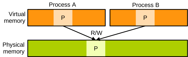
The kernel maps the same physical page within the address space of two (or more) processes. They can then read and write to that page and hit the same locations in memory.
Shared Memory: the Need for Synchronisation. When using shared memory, the fact that several processes can read and write concurrently to the same areas of memory creates the need for synchronisation. If these processes do not agree on a protocol to access this shared memory, the program may break. Imagine a scenario in which process 1 is interrupted in the middle of updating a large data structure, and then process 2 starts to run and reads that data structure while it is only half updated. This is called a race condition, and it is obviously a bug.
The issue can be illustrated as follows. We have a data structure with three fields. Initially, process 1 is running and wants to update the data structure. For it to be in a state that makes sense, all three fields should be updated. Process 1 updates the first field:
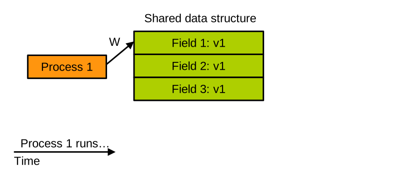
Then the second field:
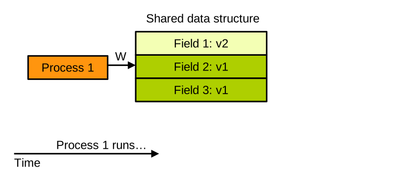
Before process 1 can update the third field, it is preempted and the scheduler decides to run process 2 on the CPU instead:
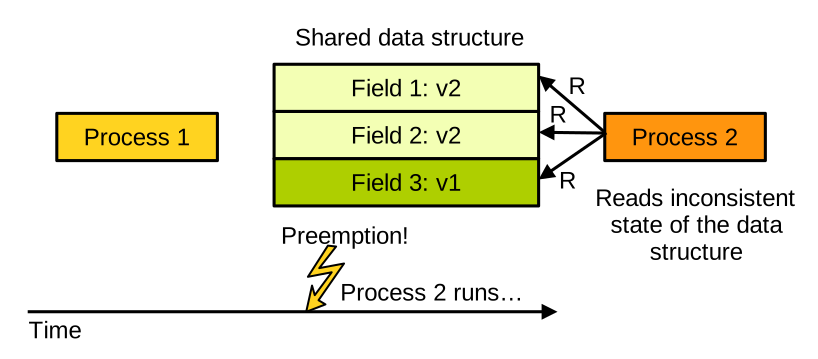
Process 2 reads the entire data structure, which is in an inconsistent state. That is our race condition.
Synchronisation
The bits of code in your program where processes access shared data are called critical sections. To avoid race conditions, the critical sections of all processes accessing a piece of shared data need to execute in a very particular fashion: they need to execute atomically. Atomicity means that these two rules must be enforced:
- A critical section can only be executed by one process at a time; and
- If a process starts to execute a critical section, it must finish it before another process can start to execute another critical section accessing the same piece of shared data.
These rules are enforced by a particular mechanism: locks.
Locks
A lock protects a piece of shared data, and works as follows. Say we have two processes that want to access some shared data, protected by one lock:

When the execution of both processes reaches the point where they need to access the shared data, each process attempts to take the lock. In its initial state the lock is free to be taken by a process, and it is implemented in such a way that only one process can succeed in taking and holding it. Let’s assume it is process 1. Because that process has obtained the lock, it can go ahead and execute its critical section, i.e. read or write the shared data: in the meantime, the second process fails to take the lock and needs to wait for it to become free again, so it is put to sleep by the OS:

When process 1 is done accessing the shared data structure, it exits its critical section and releases the lock. Process 2 then tries to take the lock again and succeeds, as the lock is now free:

Process 2 can then execute its critical section and release the lock when it is done:

This way we have ensured atomicity in the execution of the critical sections: each was executed by one process at a time, and there were no race conditions.
Locks: Example
Let’s illustrate with an example program both how to establish shared memory between two processes, and how to use a lock to protect access to data living in shared memory:
typedef struct {
    int field1;
    int field2;
    int counter;
    pthread_mutex_t lock;
} shared_data_t;

int main() {
    shared_data_t *shared;

    // Create anonymous shared memory
    shared = mmap(NULL, sizeof(shared_data_t), PROT_READ | PROT_WRITE, MAP_SHARED |
        MAP_ANONYMOUS, -1, 0);

    // Initialise process-shared mutex
    pthread_mutexattr_t attr;
    pthread_mutexattr_init(&attr);
    pthread_mutexattr_setpshared(&attr, PTHREAD_PROCESS_SHARED);
    pthread_mutexattr_destroy(&attr);

    shared->counter = 0;

    pid_t pid = fork();
    // the code below will be executed by both the parent and child processes

    for (int i = 0; i < 5; i++) {
        pthread_mutex_lock(&shared->lock); // critical section starts: take the lock

        int old = shared->counter;
        shared->field1 = rand();
        shared->field2 = rand();
        shared->counter++;
        printf("[%d] counter %d -> %d\n", getpid(), old, shared->counter);

        pthread_mutex_unlock(&shared->lock); // critical section ends: release lock

        usleep(100000); // small delay
    }

    // Wait for child in parent
    if (pid > 0) {
        wait(NULL);
        pthread_mutex_destroy(&shared->lock);
        munmap(shared, sizeof(shared_data_t));
    }

    return 0;
}
Here we first declare our shared data structure to be of type shared_data_t.
It has two integer fields field1 and field2, as well as a counter we use to keep track of the number of times the shared object is updated.
Finally, it has a lock to protect it against concurrent accesses, and the type of the lock is pthread_mutex_t.
In main, we use mmap to ask the OS for an area of memory large enough to hold our data structure.
We want it to be readable and writable (PROT_READ | PROT_WRITE), and with MAP_SHARED we indicate that it will be shared with the child process we are going to create next.
The type of lock we use here is called a mutex, which stands for mutual exclusion lock.
We indicate that it will be shared with the child process using pthread_mutexattr_setpshared.
We also set the counter of the shared object to zero.
Once this initialisation phase is done, the parent forks.
The code below the call to fork will be executed by both the parent and the child.
In a loop, they both repeat the following steps:
- First they take the lock to indicate the start of their critical section.
- Then they update the shared data structure, writing some random values in its two fields and incrementing the counter.
- And when the critical section is over, they release the lock.
When the loop is over, the parent uses the wait system call to wait for the child to exit, then cleans things up.
The lock is destroyed with pthread_mutex_destroy, and the shared memory is released to the OS with munmap.
As you can see, this program works correctly:
$ gcc lock.c -o lock
$ ./lock
[161503] counter 0 -> 1
[161504] counter 1 -> 2
[161503] counter 2 -> 3
[161504] counter 3 -> 4
[161503] counter 4 -> 5
[161504] counter 5 -> 6
[161503] counter 6 -> 7
[161504] counter 7 -> 8
[161503] counter 8 -> 9
[161504] counter 9 -> 10
[161503] final counter: 10
If you are curious about how things would run without synchronisation, you can try commenting out the pthread_mutex_lock and pthread_mutex_unlock statements to get rid of the lock.
Try running this program a few times: you will likely observe some race conditions and see the counter’s value evolve unexpectedly:
$ ./lock-with-race
[162203] counter 0 -> 1
[162204] counter 1 -> 2
[162203] counter 2 -> 3
[162204] counter 3 -> 4
[162203] counter 4 -> 5
[162204] counter 4 -> 5
[162204] counter 5 -> 6
[162203] counter 5 -> 7
[162203] counter 7 -> 8
[162204] counter 7 -> 9
[162203] final counter: 9
Locks: Implementation by the OS
The OS needs to be involved in lock taking and release operations because only the kernel can put processes to sleep or wake them up. So in the old days every lock take and release operation required a system call, which is a slow operation. This was very costly from a performance point of view.
The old way of dealing with locks, with one system call for each lock operation, is illustrated on the left here:
Linux and many other operating systems implement an optimisation to avoid involving the kernel as much as possible during lock operations. That optimisation is called futex, for fast user space mutex. It is illustrated on the right of the diagram above.
With futex, part of the lock is implemented in user space: we have a futex data structure that is accessed atomically by processes using atomic instructions. System calls are made only when the kernel needs to be involved, i.e. when a process needs to sleep or to be awakened. So when there is no contention, the lock is accessed swiftly without any system call.
Threads
Definition
A thread is an execution flow within a process.
Each process has at least one thread, corresponding to the execution flow that starts at main after the program is loaded.
A process can also create additional threads.
In C, thread creation and management are achieved with the POSIX thread library, pthread.
Threads are available in many other languages too, e.g. Python, Rust, Java, etc.
The key idea with threads is that all threads belonging to the same process share that process’ address space. This means that threads see the same global variables, and more generally they see the same value when looking at a particular slot in memory (for example through pointers). That makes it very easy for threads to communicate using global variables or pointers to anywhere in memory. Threads run concurrently, which means they also need to synchronise to avoid race conditions when accessing shared data.
Example
Here is an example of a multithreaded program:
typedef struct {
    pthread_mutex_t lock;
    int field1;
    int field2;
    int counter;
} shared_data_t;

void* thread_func(void* arg) {
    shared_data_t *shared = (shared_data_t*)arg;

    for (int i = 0; i < 5; i++) {
        pthread_mutex_lock(&shared->lock);

        int old = shared->counter;
        shared->field1 = rand();
        shared->field2 = rand();
        shared->counter++;
        printf("[%d] counter %d -> %d\n", gettid(), old, shared->counter);

        pthread_mutex_unlock(&shared->lock);

        usleep(100000);
    }

    pthread_exit(NULL);
}

int main() {
    pthread_t t1, t2;
    shared_data_t shared;
    shared.counter = 0;

    pthread_mutex_init(&shared.lock, NULL);

    // Create two threads:
    pthread_create(&t1, NULL, thread_func, &shared);
    pthread_create(&t2, NULL, thread_func, &shared);

    // Wait for both threads to finish:
    pthread_join(t1, NULL);
    pthread_join(t2, NULL);

    // Cleanup:
    pthread_mutex_destroy(&shared.lock);
    return 0;
}
That program performs the same thing as the multiprocess application we saw previously, this time with threads.
We have the same data structure with two fields, a counter, and a lock.
This time, the shared object shared is a local variable and will live on the stack of the main thread.
We also declare two pthread_t objects, t1 and t2, representing the threads we want to create.
We initialise the lock with pthread_mutex_init, then create and start the two threads with pthread_create.
The calls to pthread_create take as third parameter the name of the function the threads should run: here it is thread_func, and as fourth parameter the argument to pass to that function, here it is the address of the shared data structure.
After calling pthread_create, the main thread waits for both threads to finish with two calls to pthread_join, each taking as parameter the thread to wait for.
When they run, both threads execute the thread_func function.
It executes the same loop as our multiprocess application: take the lock, update the shared data structure, then release the lock.
See how each thread prints its own thread identifier (TID, an OS-level identifier different from the PID) with gettid().
Once they are done, each thread calls pthread_exit.
You can compile and run that example as follows:
$ gcc thread.c -o thread -lpthread
$ ./thread
[167299] counter 0 -> 1
[167298] counter 1 -> 2
[167299] counter 2 -> 3
[167298] counter 3 -> 4
[167299] counter 4 -> 5
[167298] counter 5 -> 6
[167299] counter 6 -> 7
[167298] counter 7 -> 8
[167298] counter 8 -> 9
[167299] counter 9 -> 10
The -lpthread switch instructs the linker to link our program against the pthread library.
It is unnecessary with modern versions of the GCC toolchain, but may be required when using older ones.
Implementation by the OS
Threads are created with the same system call used underneath fork: clone.
From the OS’s point of view, a thread is a task, i.e. the smallest schedulable entity.
Linux does not schedule processes, it schedules threads.
All threads of a process will report the same PID, but they also have a thread-level identifier, the TID.
Most of the scheduler-related system calls, such as the one to update priorities, actually take a TID as parameter and not a PID.
This is because threads, and not processes, are the schedulable entities.
The sharing of a single address space between all threads belonging to the same process is simple: they all use the exact same page table.
Scheduling
You can access the slides 🖼️ for this lecture.
Here we discuss scheduling, and we zoom in on the current scheduler used by Linux, the Completely Fair Scheduler (CFS).
What is OS Scheduling?
The OS scheduler in the kernel is the entity that decides what tasks should run on the CPU cores, when, and for how long. Recall that with Linux the schedulable entities are threads: we will use that term interchangeably with tasks here. Most modern operating systems support running multiple tasks at the same time; this is called multitasking. When the number of tasks is greater than the number of CPU cores, which is almost always the case in modern systems, several tasks are multiplexed in time on the same CPU core. Context switching between two tasks on a core happens very quickly, giving the user the illusion that tasks are executing in parallel.
Scheduling has several key objectives:
- Throughput: we want to run as many tasks as possible, and to minimise the overhead of running scheduling code such as context switches.
- Latency or responsiveness: when a task becomes ready to run, for example following an event such as the user pressing a button, we want it to be scheduled on the CPU as early as possible.
- Fairness: if we have several tasks with the same priority in the system, each should get an equal share of CPU time.
- Scalability: we want our scheduler to support a large number of 1) tasks and 2) cores.
Main Scheduler Classes
As you may know, there are two main classes of schedulers:
- The first one is cooperative scheduling. With a cooperative scheduler, a task won’t stop running until it decides to yield the CPU with a system call, or terminates. In that situation, the OS simply cannot enforce fairness. We could for example have a malicious task never yielding and monopolising all CPU cycles: that’s a denial of service and availability is compromised.
- The second class of schedulers is preemptive multitasking. With it, the kernel can interrupt the execution of a task; this is called preemption. Preemption can happen in various situations, for example when a task expires the amount of CPU time it was allocated by the scheduler, or when a task with a higher priority becomes ready to run. This is obviously more suitable from the security point of view with adversarial workloads.
Traditional Scheduling Algorithms
You may have already learnt in the past about some of the traditional scheduling algorithms:
- First-Come, First-Served (FCFS) or First-In, First-Out (FIFO): tasks simply run in the order they become ready until they yield or finish.
- Round-Robin: tasks run for a fixed amount of time, named a quantum, in a round-robin manner.
- Priority Scheduling: the scheduler considers priorities to rank tasks and select the one that needs to run the most.
- Multilevel Feedback Queues: tasks are divided into different priority queues, and certain types of tasks are favoured.
All of these algorithms have their pros and cons, and are great for learning about scheduling. However, none of these approaches is really efficient with modern workloads on modern machines.
We need a better scheduler for modern systems, for 2 main reasons. First, the last two decades have seen a growing number of cores integrated in CPUs. For example, it is very likely that you are reading these lectures on a computer with multiple cores. This is a scalability issue: scheduling algorithms designed to work on a single core are generally not directly compatible with CPUs having multiple cores, and other algorithms working on a handful of cores may not work that well when that number increases.
Second, the characteristics of the workloads running on modern machines have become increasingly heterogeneous. Computers run batch or background tasks that are CPU- and memory-bound, and run for a long time. Examples of such tasks are encoding videos, training ML models, etc. These jobs want to run as much as possible to keep caches warm, but they are also OK with being preempted. Conversely, we also have interactive tasks, such as text editors or video games. These are latency-sensitive: they do not need a lot of CPU cycles but need to respond quickly to certain events such as mouse clicks or pressing a key on the keyboard. Finally, in some scenarios we also have real-time tasks. These need to be schedulable in bounded time, so we can get particular guarantees. For example, soft real-time workloads such as video decoding or processing generally have quality of service requirements, e.g., keeping the frame rate above a particular threshold. Hard real-time workloads must offer safety guarantees, for example if a car’s motion sensors detect an object on the road, the brakes must be activated swiftly. All of these impose particular requirements on the scheduler.
Batch vs. Interactive Tasks
Here we have an illustration of two tasks running on a system:
One task is a video encoder, a background throughput-oriented job. The other is an interactive latency-sensitive application, a text editor. If we have a scheduler ensuring complete fairness, we would get something like what can be seen at the top, with the same amount of CPU time given to each task. That would be suboptimal, because in reality these two tasks have different needs. Indeed, the text editor only needs to run for a few CPU cycles when the user presses a key on the keyboard. The video encoder needs to run as much as possible, but is OK to be preempted by the text editor whenever needed. As a result, a scheduler realising the behaviour seen at the bottom of the illustration would be much more efficient: the goal of modern schedulers is to maintain good performance for both types of jobs, including in situations when they run alongside each other.
Linux’s Scheduler: CFS
Linux’s first scheduler dates back to the 1990s and scaled poorly to high numbers of tasks and cores. It was replaced in 2003 by the O(1) scheduler, which had the ability to take constant-time scheduling decisions, independently of the number of tasks and cores in the system. It scaled well, but had some issues with latency-sensitive interactive tasks.
The current scheduler on Linux is the Completely Fair Scheduler, CFS. It was introduced in Linux 2.6.23 in 2007.
CFS: Core Idea
To understand how CFS works, first assume a CPU with only a single core for the sake of simplicity. CFS defines a fixed time interval during which each thread in the system must run at least once. This interval is split into timeslices, 1 per thread. The length of the timeslice for each thread is proportional to the thread’s weight, which is basically its priority, also named the nice value in Linux.
The scheduler keeps track of how much time each thread spends on the CPU. That time, divided by the thread’s weight, gives what is called the vruntime for that thread.
CFS decides to preempt a thread running on the CPU when that thread exceeds its timeslice and there are other threads ready to run. A running thread is also preempted when another thread with a smaller vruntime wakes up.
CFS Runqueues
To achieve these scheduling decisions, CFS organises all threads that are ready to run into a runqueue, which is a red-black tree:
Each node in the tree is a thread ready to run. They are sorted in the tree by increasing order of vruntime. This way, it is easy for CFS to pick the next task to run: it always corresponds to the leftmost node. Using a red-black tree also allows CFS to have low performance overheads. Indeed, things like inserting and removing nodes, rebalancing and recoloring the tree, are realised with O(log n) complexity.
On a multicore CPU, CFS has 1 runqueue (1 red-black tree) per core in the system. This way, the vast majority of scheduling decisions can be made locally in a per-core manner. They do not necessitate inter-core communication, which would require synchronisation with mechanisms such as locks, and would slow things down too much.
Still, the per-core runqueues must be kept balanced: we don’t want to end up in situations with 1 core having many high-priority threads and the other cores with just a few low-priority threads in their runqueues. To address that problem, CFS implements a relatively complex load balancing algorithm, that moves threads between the runqueues of different cores to balance things. This algorithm considers the threads’ priorities, the number of threads in each runqueue, but also the system’s topology, including the cache hierarchy, hyperthreading, and NUMA nodes. Indeed, there is a cost in migrating a thread away: for example, it will have to rebuild its local cache state on the target core.
vruntime Explained
The vruntime value for each thread, which is used to rank them in the runqueue, is weighted by their nice value.
A thread’s nice value is basically an inverted priority metric: the higher the nice value, the nicer the thread is, i.e. the more it is OK to let other threads run.
The way the vruntime is computed for each thread ensures that long-running CPU-intensive threads will see their vruntime increase faster, giving more chances to run for I/O bound/interactive threads, that do not run much, when these become ready.
Preemption and Context Switches
With Linux, preemption works as follows. When the scheduler decides that the currently-running thread should be preempted, it sets a per-CPU flag to indicate that. Remember that this happens when the running thread exceeds its timeslice, or when a thread with a higher priority (with CFS, a lower vruntime) wakes up and becomes ready to run. The thread in question is not immediately preempted. Instead, the flag is checked by the kernel before returning to user space, for example following a system call, exception, or hardware interrupt. If the flag is set, preemption happens and a context switch is performed. The kernel switches the CPU context to that of the target thread. We have seen previously how a context switch is done: the content of the CPU registers is dumped to memory to save the execution context of the task being scheduled out, and the CPU registers’ content is set with the execution context of the task being scheduled in. That includes a control register that indicates which page table should be used; in effect, this switches the address space to that of the target thread.
Security Aspects
There are some security aspects to scheduling. An attacker taking control of a user-space application can issue scheduling-related system calls and manipulate some scheduling parameters. They could set a higher priority or a prioritised scheduling policy on malicious threads, in order to compromise the availability of other applications.
The solution to that issue is to prevent untrusted users from accessing scheduling parameters. We will see later approaches for filtering the system calls that can be issued by an application that is not trusted. There are also additional CPU isolation mechanisms, in particular a subsystem called control groups on Linux, which is used by containers. Control groups allow setting CPU quotas for threads, which are independent of the scheduling policy used. We will talk about control groups in more detail when we cover virtualisation.
Memory Management
You can access the slides 🖼️ for this lecture.
Here we cover another key responsibility of operating systems, memory management. It corresponds to the set of features implemented by the operating system to manage memory allocation, protection, and accesses. Features that fall under memory management are:
- Memory allocation/deallocation for applications and for the kernel.
- Setting up and maintaining address spaces for processes and for the kernel.
- Enforcing memory protection (isolation) between processes and the kernel, and in between processes.
- Swapping (saving memory content to disk).
- Etc.
Virtual Memory
As you know, the CPU accesses memory with load and store instructions. In the vast majority of modern systems, the CPU enables virtual memory early during the boot process. From that moment, all the addresses targeted by loads and stores will be virtual, and the CPU will no longer be able to address physical memory directly. The translation between the virtual addresses the CPU requests to access and the actual physical memory they correspond to is done transparently by the MMU:
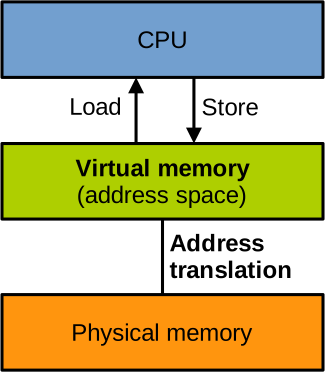
Segmentation
An old implementation of virtual memory is segmentation. An application will get access to a relatively small virtual address space, a segment, whose size is a subset of the total RAM size. That address space is then mapped to physical memory contiguously. In effect, the address translation just consists in adding an offset to a virtual address to obtain the corresponding physical one.
Below you can see an illustration of a CPU accessing memory with segmentation when an application App. 1 runs (left) and when another application App. 2 runs (right):
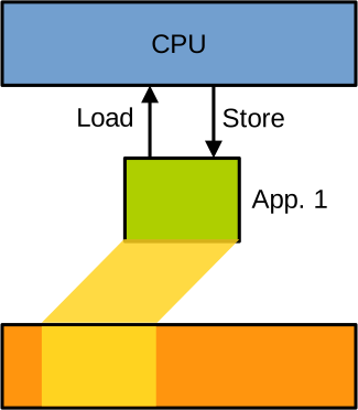
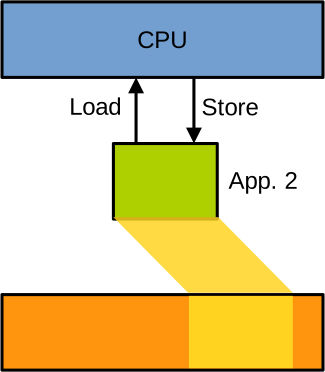
Each application has its own address space defined by a segment base address in physical memory, and a size. To ensure that the applications are isolated, the OS makes sure that the physical memory accessible through such address spaces is non-overlapping. The translation is realised simply by adding the base address as an offset to each virtual address to obtain the corresponding physical address. Overall segmentation was not very flexible. In particular, the requirement to have each address space map to a contiguous area of physical memory brought fragmentation issues.
Paging
Rather than segmentation, the vast majority of modern systems use paging to implement virtual memory. With paging, almost the entire space addressable given the width of the memory address bus is accessible to make up each process address space. For example, on most Intel 64-bit CPUs virtual addresses are 48 bits wide, which gives a virtual address space of 256 TB for each process. Of course, most of that address space is not mapped to physical memory. With paging, the mapping is achieved at the granularity of 4 KB pages. A data structure called the page table defines what virtual pages are mapped to physical memory, and where to:
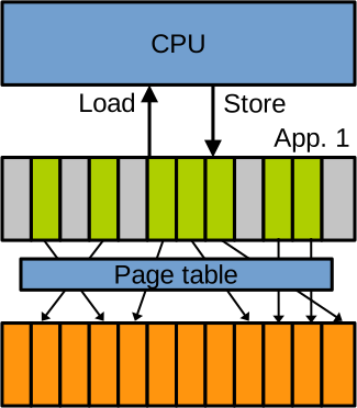
Each process has a different page table, and without establishing shared memory processes do not share physical pages. This way they are fully isolated from each other. Concretely, the way a page table handling the address space of a process works is as follows:
- The OS sets up the page table when the process is created. The OS also maintains the page table when new mappings need to be added/removed, for example when the process loads a shared library or allocates memory.
- A page table installed is walked transparently by the MMU to achieve the translation when the CPU runs the process in question and accesses memory.
The Page Table
The page table itself is implemented as a tree living in physical memory. Using a linear array with one entry per virtual page would be highly inefficient, as modern 64-bit address spaces are very large, there are many pages, but most of them are not mapped. The tree is made of pointers linking together special pages in physical memory used for address translation. Using a tree means that the system can avoid storing a lot of translation information corresponding to the large areas of the address space that are not mapped to physical memory. On modern CPUs the page table generally has 4 levels of pointers, although we are starting to see some CPUs with 5. The address of the root of the tree is held in a specific control register, so to change address space during context switch the hardware simply switches that register to the root of the page table for the process being scheduled in.
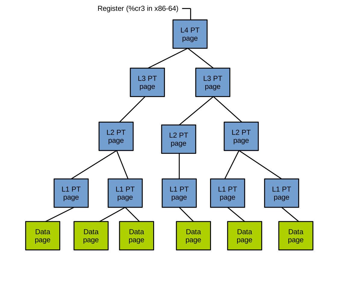
The diagram above illustrates a typical 4-level page table.
The address of the root page is held in a control register on the CPU; for Intel x86-64 this is %cr3.
The root node represents the 4th level of the page table, and the entries it contains reference pages of the 3rd level.
Entries at the 3rd level reference pages of the 2nd level, and their entries reference pages of the 1st level.
Finally, entries at the 1st level reference the physical pages holding the data accessed by the CPU.
As I mentioned, each translation page contains pointers to the next level. The size of a page is 4 KB, so there is enough space for 512 pointers:
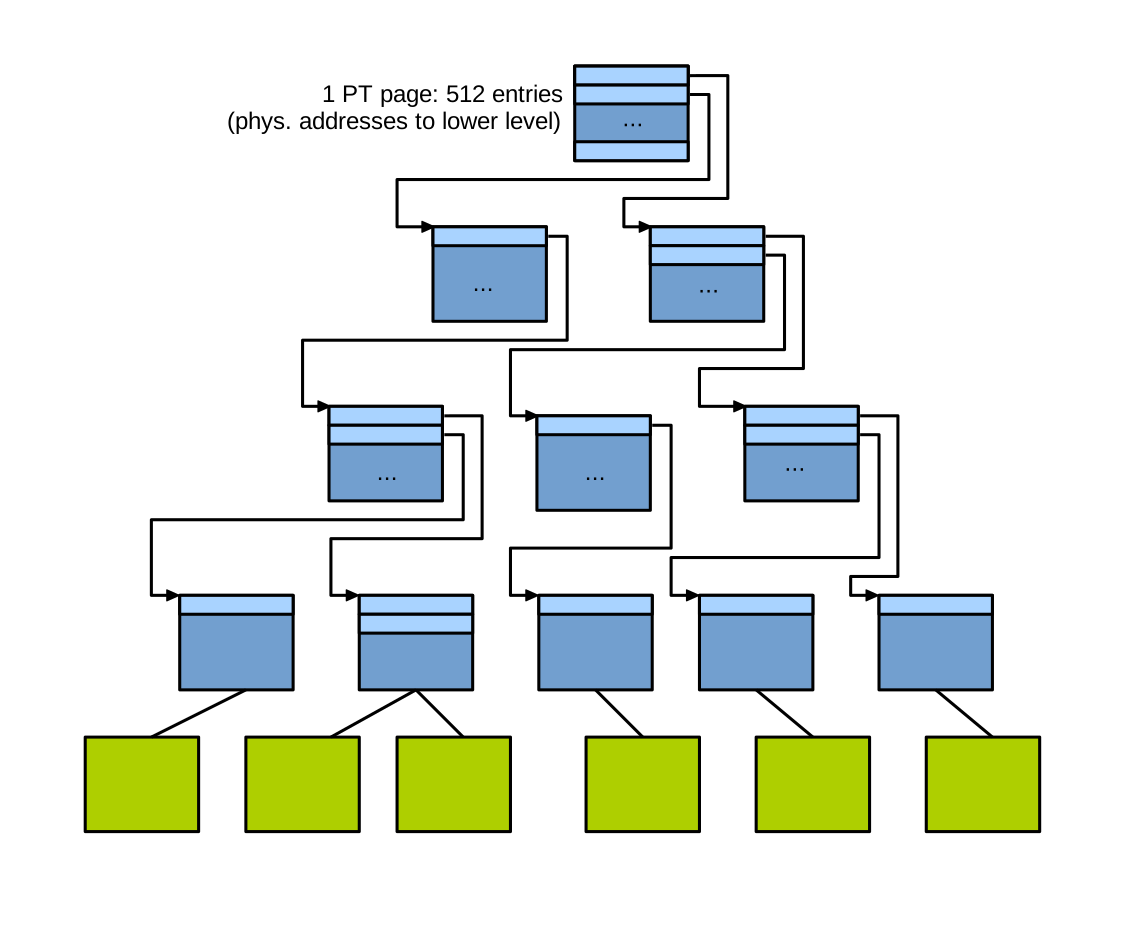
Each pointer may be either present, meaning it corresponds to a range of virtual address space that is mapped, and its value refers to a page at the lower level. Or absent, meaning it corresponds to a range of the virtual address space that is not mapped. Note that all pointers in translation pages refer to physical addresses.
Page Table Walk
When a page table is installed and the CPU issues loads and stores, the page table is walked transparently by the MMU to perform the translation.
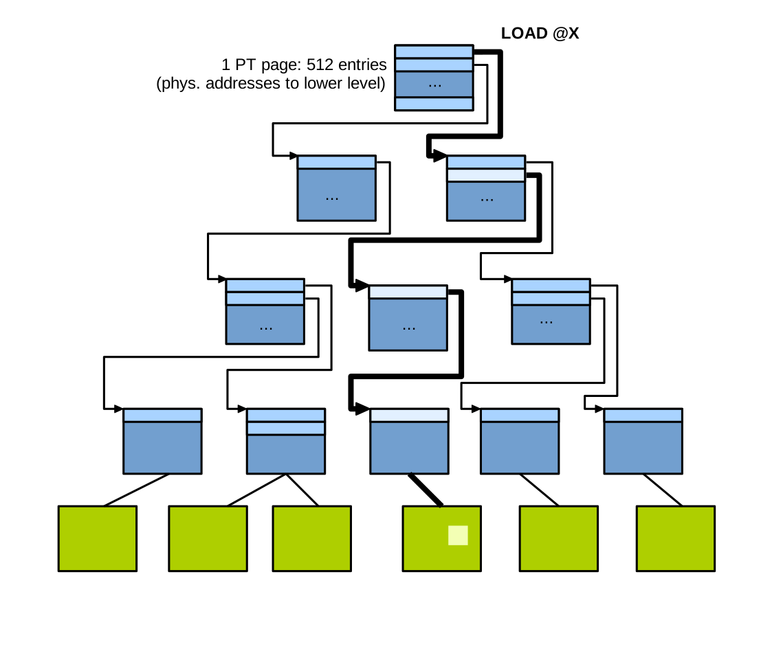
For example, if the CPU issues a load at address x, the MMU follows the path of pointers indexed by x, and the data read by this load operation will be the byte hit in the data page at the end of the walk.
To see how the entries in the page table are indexed during a page table walk, consider the following 64-bit virtual address, depicted in binary on the slide. A page table walk is performed transparently by the MMU, as follows:
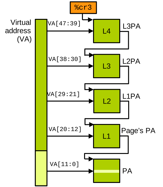
On x86-64, the %cr3 control register holds the address of the root of the page table, which is the 4th level.
The bits 39 to 47 of the target virtual address are used to index an entry in the root page, which gives us the pointer to the 3rd level translation page.
Then the bits 30 to 38 of the target virtual address index an entry in the 3rd level translation page, which gives us the pointer to the 2nd level page.
The bits 21 to 29 of the virtual address index an entry in the 2nd level translation page, giving the pointer to the 1st level page.
The bits 12 to 20 of the virtual address index an entry in the 1st level translation page, giving the pointer to the physical page the CPU wants to access.
And finally the last bits of the virtual address, bits 0 to 11, index a byte within that physical page.
Page Table Entries (x86-64)
As previously mentioned, each page composing the page table contains 512 entries, each of size 64 bits. The entirety of the 64 bits of an entry are not needed to index the lower levels. First, on most 64-bit processors the virtual address space is rather indexed on 48 bits. Second, the pointers in the translation page do not refer exactly to physical addresses, but rather to physical page indexes. Obviously there are fewer physical pages than there are physical addresses, so we need fewer bits to index them. Overall, we only need 36 bits for each entry, and we can use the additional bits to hold metadata about the range of the virtual address space referenced by each entry in translation pages:

This metadata is used to indicate whether the range of address space concerned is actually mapped, whether it is accessible in read and/or write mode, and whether it is accessible in user mode or only in supervisor mode. This allows to control memory accesses: if the address in the virtual address space is not present, or if the access in question is denied — for example because the page is read-only and the access is a write — the CPU will trigger a page fault exception. This is crucial to the security of the system, and it is used to implement memory protection, but also things like swap and the on-demand duplication of the address space upon fork.
The OS and the Address Space
Because the page table entries carry a bit that can mark part of the address space as accessible in supervisor mode only, the kernel can actually live in the same address space as processes. On Linux, the kernel is mapped in the top part of the address space of each process:
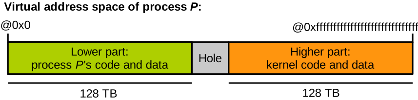
Every page table is configured so that this area is accessible in supervisor mode only, i.e. by the kernel only. This has an important advantage: there is no need to switch page tables upon system calls. Switching page tables is very costly in terms of performance, because it involves a flush of the translation cache, the translation lookaside buffer (TLB).
To sum up, the mechanisms enforcing the main memory security invariants in the system are twofold:
- Processes are isolated from each other by having different page tables defining different, non-overlapping address spaces.
- The kernel is isolated from processes through the supervisor-only access bit in each page table.
The Kernel Address Space
If we zoom in on the part of the address space reserved for the kernel, it is made of many different areas:

We cannot go over each area here, but here are the main ones:
- The dirmap is a direct linear mapping of all physical memory. It is useful when the kernel wants to access physical memory directly, for example when setting up page tables, or when allocating memory that needs to be contiguous in physical memory.
- The vmalloc area is basically the kernel heap, containing memory allocated dynamically.
- As with a standard program, the kernel also has a static memory part with its code and static data; these were mapped from the kernel’s binary at boot time.
- Finally, Linux supports the dynamic loading and unloading of kernel code at runtime, in the form of kernel modules. These are loaded in a specific area of the kernel part of the address space.
Memory Allocation in the Kernel
When the kernel needs to allocate memory for itself or for an application, the following steps are required. The kernel first reserves some physical memory, enough space to satisfy the allocation request. It also needs to find a free range of virtual memory, either within its own area of the address space if the allocation request originates from the kernel, or within the process-accessible part of the address space if it is a process requesting memory. The kernel then creates the page table entries corresponding to the newly created virtual pages, and these page table entries are set up to point to the physical pages that were previously reserved. In many cases, this mapping is not performed at allocation time, but rather later, when the CPU accesses the virtual pages for the first time. This is achieved by leaving the present bit unset in the page table entries: the first access will trigger a page fault, and at that time the kernel can perform the mapping and restart the memory access. The memory allocation request finally returns a pointer to the newly allocated virtual area that the kernel or application can use to access the memory in question:
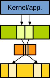
On the top of the diagram above we have the kernel or an application accessing an area of virtual memory (2 pages in green for that example). These pages are mapped to physical pages (in yellow) through the page table (in orange), which contains one page table entry per virtual page to map.
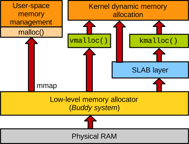
All requests for memory allocations in the system are served by the kernel.
If they come from user space (such as malloc on the diagram above), they are made through the mmap system call.
Note that malloc is implemented in user space by the libc, which in turn calls mmap under the hood to obtain a large area of virtual memory.
The malloc implementation in the libc then manages that area by splitting it into smaller buffers to serve allocation requests.
kmalloc and vmalloc
The kernel often needs to dynamically allocate memory for itself. To that end it provides two main interfaces, illustrated in green in the diagram above:
kmalloc, used for fast, small-sized allocations. It is usable in contexts where kernel code cannot sleep, for example when handling an interrupt. It also returns memory that is already mapped and always physically contiguous, which is important in particular scenarios such as allocating memory that is supposed to be accessed by devices.vmalloc, used for larger allocations at page granularity. It is slower as it requires updating the page table, and does not necessarily allocate memory that is physically contiguous.
SLAB Allocator
kmalloc relies on the SLAB layer which is a system of caches trying to reuse same-size allocations as much as possible.
This is good for speed, but also it reduces fragmentation.
It is useful when many data structures of the same type are allocated frequently.
Kernel code can also directly create its own SLAB caches without going through kmalloc.
Physical Page Allocator
To reserve physical memory, all allocation methods rely on the buddy system, also called the frame allocator. Here a frame means a physical page. This is the granularity at which the buddy system allocates physical memory. The buddy system maintains lists of blocks of same-size sets of contiguous free physical pages, with the goal of limiting fragmentation. Large blocks can be split and merged as needed. This can be illustrated as follows:
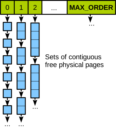
You can see the way the buddy system works here, with lists linking blocks of 1, 2, 4, 8, etc. contiguous physical pages.
Operating Systems Part 1: Further Readings
Operating Systems: General Concepts
Many books have been writen on operating systems, some of the most popular are:
- (book) Tanenbaum and Bos, Modern Operating Systems.
- (book) Silberschatz et al., Operating System Concepts.
- (book) R. Arpaci-Dusseau and A. Arpaci-Dusseau, Operating Systems: Three Easy Pieces. Very user-friendly, available for free in PDF here.
Linux Internals and Kernel Programming
- (book) Love, Linux Kernel Development. A bit oldish but very beginner friendly. Great to get started with kernel development.
- 0xAX, Linux Insides. deep but guided dive into many aspects of Linux’s source code.
- Linux Foundation, A Beginner’s Guide to Linux Kernel Development.
- (book) Bovet and Cesati, Understanding the Linux Kernel. Quite old.
- (book) Mauerer, Professional Linux Kernel Architecture.
Linux Systems Programming
Systems programming is the development of low level, user space applications that call the OS interface (system calls, and other low level primitives such as fork, mmap, IPCs, etc.) relatively directly.
- (book) Kerrisk, The Linux Programming Interface.
- (book) Love, Linux System Programming.
Miscellaneous
- OSDev Wiki, System Calls page.
- Lozi et al., The Linux Scheduler: a Decade of Wasted Cores.
- (book) Gorman, Understanding the Linux Virtual Memory Manager.
Storage and Network: Brief Introduction
You can access the slides 🖼️ for this lecture.
Here we talk about the last two important features of operating systems we cover in this unit: storage and networking.
Computer Input/Output
A computer consists of a CPU, some memory, as well as I/O devices. The two I/O devices you’ll find in almost every computer are a secondary storage device, and a network card. There are some types of computers, such as servers, that don’t really have any other I/O apart from networking and storage. Same for many embedded devices: there is no mouse, no keyboard, no screen; however, they still need storage for persistence, and some form of access to the network for communication with the rest of the world.
Here we will see a brief introduction to how storage and networking work with Linux. We cannot go into too many details for time reasons, but there is much to say about storage and networking: these are very deep and complex topics, and there are entire books focusing on each.
The Linux Storage Stack
This is a simplified overview of the Linux storage stack:
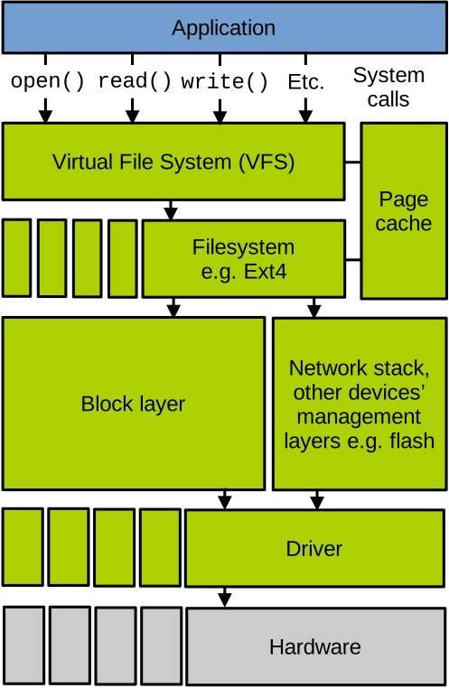
We have the application on top, and each layer of the operating system involved in storage management, down to the hardware. You may have heard of the fundamental theorem of software engineering, which states that “we can solve any problem by introducing an extra level of indirection”. The storage stack is a good illustration of this. Let’s go over these layers one by one.
System Calls and VFS Layer.
Like every other operating system service, applications access storage using system calls.
You know the filesystem-related ones: open, read, write, lseek, etc.
These system calls are received by the topmost layer of the storage stack in the OS: the Virtual File System (VFS). Its goal is to abstract all filesystems supported by Linux under a common interface, which is the set of system calls we just mentioned. These system calls are translated by VFS into concrete filesystem operations. VFS allows mounting multiple filesystems in a single directory tree. The benefits to having a unified interface to access files sitting on different filesystems are quite obvious: applications can be written independently of the filesystem used to store the files they access. Finally, VFS factorises a lot of storage management code that does not need to be implemented on a per-filesystem basis. This is particularly true for data and metadata caching code.
File System Layer.
Below VFS we have the concrete filesystems.
The filesystem’s implementation defines concretely how file data and metadata are stored and retrieved from the storage device.
Linux supports tens of filesystems.
Many target traditional storage devices such as hard disks and SSDs, but we also have RAM-based filesystems, pseudo filesystems that do not store any data (for example /proc and /sys), network filesystems (e.g., NFS), as well as filesystems for other media such as optical disks, embedded flash chips, etc.
Page Cache. Connected to the virtual and concrete filesystem layers, the page cache is the main file data cache on Linux. File data that is read is cached in RAM in case it needs to be read again in the future. File data that is written is cached in RAM for a bit of time to buffer short-term bursts of write requests before flushing them to disk. Linux’s policy on how much RAM to use for caching file data is simple: all the RAM that is not used by running programs and the kernel can be used to cache file data. The goal is to maximise the usage of your RAM.
We can check how much of your RAM is used to cache file data with this command:
$ free -h
               total        used        free      shared  buff/cache   available
Mem:            15Gi       5,2Gi       2,8Gi       179Mi       8,4Gi        10Gi
Swap:           15Gi          0B        15Gi
The amount of main memory used for the page cache is indicated by buff/cache: it is common to see gigabytes of RAM used for that purpose.
Block Layer. Below the filesystem we have the block layer. It is another indirection layer that abstracts block devices, i.e., storage devices accessed at relatively large granularities. For example, most hard disks are accessed at the granularity of a sector, which is 512 bytes. In addition to providing a common interface for all block devices, the block layer implements block I/O request schedulers that will queue, reorder, merge, or split requests to maximise performance. For example, one of the main goals of hard disk I/O schedulers is to avoid moving the magnetic head of the disk, which is a very costly operation.
Device Mapper. The block layer also allows creating virtual block devices on top of physical ones, to implement in software some features not always supported by the hardware, such as encryption, virtual partitions, compression, caching, aggregation of multiple disks for performance and fault tolerance reasons, etc. This is achieved through a layer called the device mapper.
Non-Block Storage. There are also quite a lot of filesystems and other storage layers that do not target block devices. For example, NFS will fetch the filesystem and propagate modifications through the network. Another example concerns the management of the embedded flash chips that can be found on early smartphones, which is realised by a dedicated subsystem named Memory Technology Device.
Drivers & Low-Level Layers. Between the block layer and the driver there may be more abstraction and protocol layers, such as USB, SCSI, SATA or NVMe. The lowest level of software in the storage stack corresponds to the device drivers. Drivers are in charge of sending to the device the I/O requests submitted by the higher layers. Generally, there is one driver per model of device, and Linux supports a very high number of devices. In fact, more than two-thirds of the 20 million lines of code that make up the kernel correspond to device driver code.
VFS Data Structures
We can zoom in a little on the VFS layer, which is the filesystem abstraction layer that handles system calls from user space directly. It uses a series of data structures to handle filesystem operations. Some are created when a disk partition hosting a particular filesystem is mounted. Others are created on demand when filesystem objects are accessed, for example when a file is opened. These data structures are used by VFS, and they are generally created by the concrete filesystem itself because only the filesystem knows how file data and metadata are stored on the storage device; VFS is just an abstraction layer.
These data structures can be represented as follows:
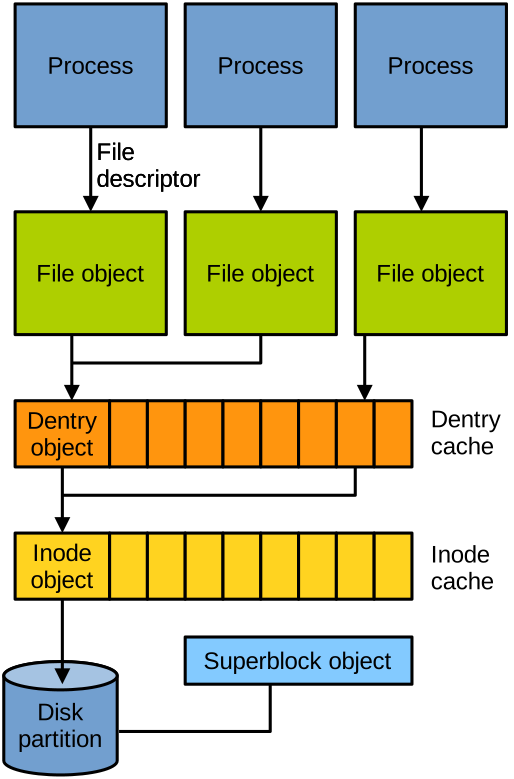
Superblock. A first interesting object is the superblock. There is one instance of this object per mounted filesystem; here, by filesystem, we mean a partition. The superblock contains general information about the partition, such as the filesystem type, mount flags, etc. It exposes a series of methods to execute partition-level operations such as flushing caches or unmounting the partition.
Inodes. A key data structure for filesystems is the inode. There is one inode object per file or directory on the filesystem. It contains metadata about the file, such as its size, owner, and permissions. Inode objects are created by the concrete filesystem and buffered in RAM in what is called the inode cache. They expose methods to perform file-level operations: creating, deleting, resizing, moving files, etc.
Directory Entries. A file’s name and location in the directory tree are not contained in the inode, but instead in a dedicated data structure which is called a directory entry (dentry). Dentries are used for operations on the directory tree, such as pathname lookup or listing the content of a directory, and they expose methods to accomplish these operations. Dentries are buffered in RAM in what is called the dentry cache. There is at least one dentry per file or directory in the filesystem, and there can be more than one in case you create hard links.
File Objects. Finally, the file object represents an instance of a file opened by a process. Each file descriptor used by the program corresponds to a file object in the kernel, so you can have several file objects for the same file if that file is opened multiple times by the program. The file object holds metadata about the opened file, for example, the file offset or the flags it was opened with. The file object exposes methods to access the file: reading it, writing it, etc.
Networking
Brief Overview
Let us now very briefly talk about the network stack. An ultra-simplified diagram depicting it is below:
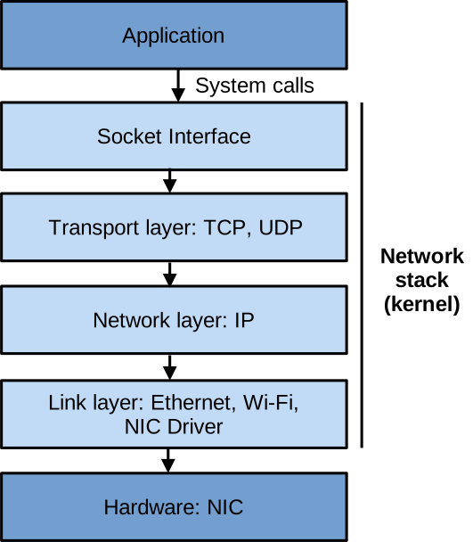
Once again remember that this is a very brief, high-level overview, as we do not have time to go into many details here. The network stack is composed of the following layers:
System Calls and Socket Interface.
Similar to all other OS services, applications access the network through system calls, such as socket, connect, listen, etc.
These network-related system calls form the socket interface.
They let an application create a server listening on a port, and send/receive data with system calls that are akin to reading from and writing to files.
Transport Layer. Below the socket interface we have the transport layer, implementing transport protocols – the main ones being TCP and UDP. This layer splits or assembles data to send and receive into packets and handles things like reliability, ordering, and flow control.
Network Layer. Below that you have the network layer, which is in charge of figuring out where each packet should go. So it takes care of addressing and routing. Here, generally, the protocol used is IP.
Link Layer. Finally, we have the link layer that handles things like physical addressing, and that also contains the network card driver.
Going Further
Beyond this brief overview, to learn more about the Linux network stack, feel free to consult the following resources:
- Rami Rosen, Linux Kernel Networking Implementation and Theory
- Christian Benvenuti, Understanding Linux Network Internals
OS Security Concepts
You can access the slides 🖼️ for this lecture.
Introduction
We have previously covered the many responsibilities of the OS, which is a foundational component of modern computer systems. As such, the OS plays a key role in the security of the computer system it controls. The primary security goals of an OS include enforcing which operations (e.g. read, write) subjects (e.g. applications, users) can perform on objects (e.g. files, system resources), applying the principle of least privilege to maintain confidentiality, integrity, and/or availability. These security goals are often at odds with other OS objectives such as performance, resource usage, convenience of use, or compatibility.
Fundamental OS Security Invariants
The two main entities to which the permissions/restrictions considered in OS-enforced security policies are applied are processes and users. We have already seen the following process-level fundamental security invariants an OS aims to maintain:
-
Inter-Process Isolation. By default, processes should not be able to access (in read, write or execution mode) each other’s state (mostly memory) directly. We have seen that this is enforced with virtual memory, by giving each process its own virtual address space. In most modern CPUs this is realised with the page tables defining non-overlapping virtual address spaces for processes.
-
User/kernel isolation. Processes should not be able to access the memory reserved for the kernel directly. To request services, processes can only invoke the kernel at a safe and well-defined entry point. These two security objectives are achieved with the user/supervisor execution mode and associated bits in page table entries, as well as the system call mechanism.
In addition to the process-level invariants, the OS enforces several user-level security invariants:
-
User authentication. Only authorised users should be able to access the system. This is enforced with authentication mechanisms such as passwords, biometric identifiers (fingerprint, face ID), or other credential-based approaches.
-
User-controlled resource sharing. Users must be able to configure how to share or not share the resources they own with other users. In UNIX/Linux systems, this is primarily implemented with file permissions, where files abstract many types of system resources.
-
Privileged operations. Only privileged users (administrators) should be able to accomplish security-critical tasks such as loading kernel code, shutting down the computer, mounting filesystems, or modifying system-wide configurations.
A Basic OS Trust Model
When considering the security of a computer system from the OS point of view, the trust model we have assumed so far is as follows: the entirety of the OS kernel is trusted, and local user space applications are not trusted. Remote applications (e.g., clients connecting to a server hosted by the system) are not trusted either. Similarly, local or remote non-administrator users are not trusted. This trust model can be illustrated as follows:
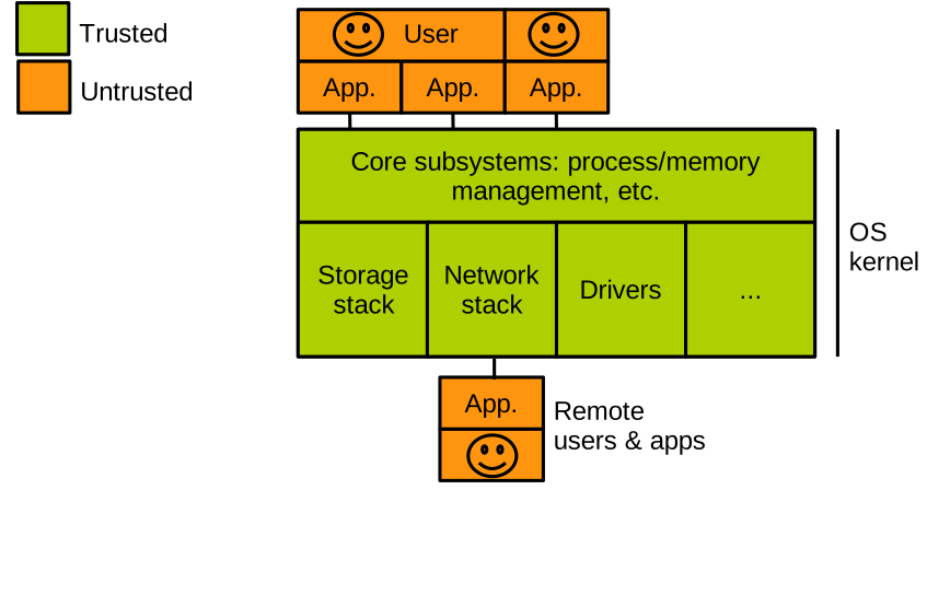
In reality, this model is overly simplistic and does not consider components of the system that are key to its security:
- The hardware, which is assumed by the OS to behave correctly for any kind of security guarantee to hold in the system.
- The system administrator has ambient authority over the system: should they be malicious, the OS security guarantees simply cannot be maintained. Further, certain applications (e.g., programs logging users in, or changing users’ passwords) are privileged. If one of these is compromised, the aforementioned OS security invariants are likely to break.
- The system’s components involved in the boot process are also assumed to behave properly. That includes the motherboard’s firmware, the BIOS, bootloader, and OS boot process. Once again, if a component of the boot process is compromised, the system cannot be secure.
All these components are fully trusted in the OS trust model we have considered so far. A more complete illustration of that model, taking into account the components we just covered, is as follows:
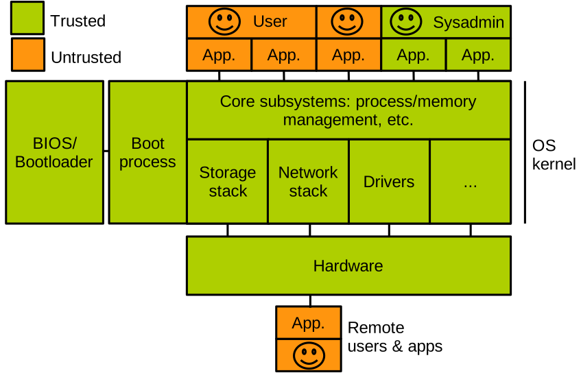
The large quantity of green boxes in that diagram should give you an idea of the immense amount of software and hardware that is blindly trusted to work correctly when considering the security of a computer system. This raises the following question: does this trust model reflect the reality of today’s computer systems?
Realistic OS Trust Model
The answer to the previous question is no. It is easy to identify situations in which the components that are assumed trusted in our basic trust model may actually be faulty or malicious. The BIOS, bootloader, or other boot process software may have bugs or be corrupted. A local attacker could swap the on-disk kernel image, loaded at boot time, with a malicious one, or install a bootkit. The OS kernel itself is not exempt from bugs and vulnerabilities. This is particularly problematic in subsystems developed by third parties (e.g., drivers), which may not have the same degree of code writing quality, secure coding practices, or testing/validation discipline as core kernel subsystems. The hardware itself cannot be fully trusted, as it presents faults and vulnerabilities, see for example the Spectre and Meltdown micro-architectural side channels identified in 2017. Finally, the system administrator or the owner of the computer an application executes upon may not be fully trusted: for example, one of the reasons certain businesses refuse to offload some of their internal workloads to the cloud is because they do not trust the cloud providers with access to their data.
In that context, a more realistic OS trust model can be represented as follows:
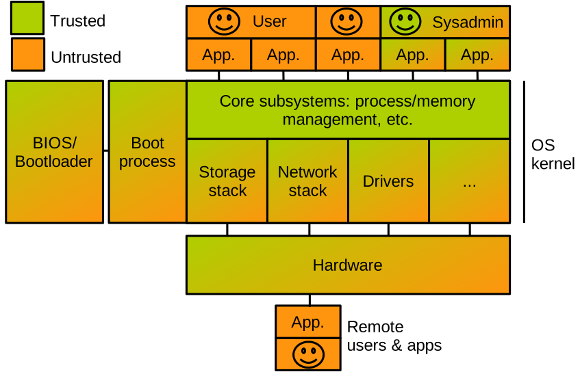
Security concerns regarding the hardware, boot process, system administrator, or internal untrusted components of the OS have been the target of several recent technologies and protection techniques, which will be covered in the remainder of this course unit:
- The lecture materials on trusted execution environments will consider scenarios where the system administrator/host computer is not trusted.
- The part on software compartmentalisation will cover how to isolate untrusted components of applications and operating systems.
- Finally, the hardware part of the unit will discuss hardware security and secure boot.
Application - Kernel Isolation
Let us zoom in on the isolation of the kernel from applications. For that we can simply consider the following basic trust model: applications distrust each other and trust the kernel, and the kernel distrusts applications:
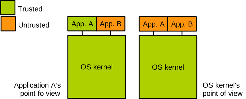
We have seen earlier that one of the main security invariants an OS aims to maintain is inter-process isolation: applications should be isolated from each other. This is relatively intuitive: some applications in the system perform security-sensitive tasks (e.g., authenticating a user, installing new software, etc.) and handle critical data (check the validity of a password, generate and process crypto keys, etc.) while other applications are not fully trusted (they may run on behalf of an untrusted user, be faulty, or under the control of an attacker and plainly malicious) and it makes sense to isolate both classes of programs. Because it is often difficult to determine if an application is security-sensitive or is not to be fully trusted, OSes implement a policy that is safe by design: by default, each process running in the system should be isolated from the other processes.
We have also seen that the kernel is in charge of enforcing the isolation across processes, by setting up their page tables and defining their virtual address spaces to be non-overlapping. For that reason we need the kernel to be isolated from applications: this is our second security invariant. If an application could modify or access the kernel’s memory, for example, to modify page tables or run code that allows updating memory mappings, our cross-process isolation security invariant would break.
User -> Kernel Attacks
Although the kernel is well isolated from applications, these still need to be able to invoke the kernel to perform system calls: although this is made through a controlled interface, this interface still raises security concerns. Production-ready kernels such as Linux are written in memory unsafe languages, so they are subject to all the memory safety and undefined behaviour vulnerabilities we saw previously. Due to their sheer size, millions of lines of code, we cannot rule out the possibility of bugs and vulnerabilities in these OSes, for example on the processing path of system calls. Hence, although processes cannot access each other’s memory directly, a process triggering a bug in the kernel through the invocation of one or several system calls may be able to mislead the kernel into interfering with or accessing the memory of another process: from the kernel’s point of view, the system call interface is a primary attack vector:
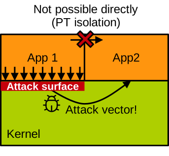
This is particularly concerning as the system call interface is extremely large and complex. Linux has more than 350 system calls, some of them implementing up to thousands of sub-functionalities, e.g., \texttt{ioctl}. Because of that size and complexity, that interface is very difficult to fully secure, and we cannot rule out the possibility of kernel bugs and vulnerabilities triggered by applications using that interface.
Hardening The System Call Interface
Because the system call interface is the main user -> kernel attack vector, the OS considers every piece of data flowing from user space to the kernel through system calls as untrusted. That includes system call parameters and, for pointer parameters, what they point to. In that context the kernel must protect itself against the user space injecting:
- Corrupted data structures
- Bad indexing information
NULLpointers- References to resources (e.g., files) that the process does not have permission to access
- Sequences of system call invocations in the wrong order
- Etc.
The kernel must sanity check the validity of the system call data and control flow coming from user space. As mentioned earlier, getting these checks 100% correct is difficult due to the size and complexity of the system call interface.
Sanity Checking System Call Pointer Parameters
A process often passes a pointer to some of its memory to the kernel.
Consider for example the readv system call:
ssize_t readv(int fildes, const struct iovec *iov, int iovcnt);
This system call performs several (iovcnt) read operations from a file identified by a file descriptor filedes.
The operations are described in an array of iovec vector data structures which is located within the application’s address space, and passed to the kernel as a reference iov.
That pointer could be invalid, and the content it points to could be corrupted: for safety reasons, before accessing that array the kernel needs to check the validity of the pointer (e.g., is it NULL?) and of the content it points to.
These validity checks depend on the data structure in question, for iovec elements Linux will check that each vector’s length is not negative and will not overflow the target buffer, that the pointers to target buffers are valid and point to user-accessible memory, etc.
These sanity checks cannot be made directly to the area of user space memory referenced by system call pointer parameters. This would open the kernel for a type of vulnerabilities called Time of Check to Time of Use (TOCTTOU), also known as double fetch. Assume that sanity checks are made by the kernel directly in user space memory and consider the following scenario:
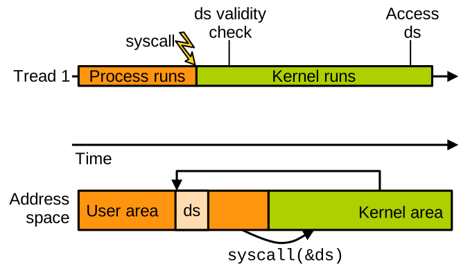
We have a view in time of what runs on the CPU on top, and a memory view at the bottom. A thread of an application runs on a CPU core and invokes a system call with a pointer parameter referencing a data structure in user space. The kernel takes over, sanity checks the data structure, and if the check succeeds, the kernel can access the data structure: all is well.
With this scenario, a TOCTTOU attack works as follows: the user space application can use another thread to corrupt the data structure after the check, but before the kernel accesses it:
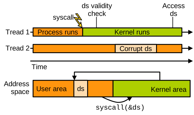
This can be done if the application’s code can run concurrently with the kernel: corrupting the data can be done from another thread, a signal handler, or from another application sharing the area of memory in question. In effect, this attack can bypass the sanity checks made by the kernel. The solution implemented by modern kernels to protect against TOCTTOU issues is to copy into kernel space all user space data passed by reference. Validity checks can then be performed on these copies, which cannot be accessed by user space at all:
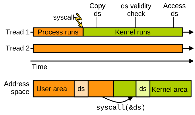
To perform these copies, the kernel uses two functions:
unsigned long __copy_from_user(void * to, const void __user * from, unsigned long n);
unsigned long __copy_to_user(void __user * to, const void * from, unsigned long n);
__copy_from_user copies n bytes of memory from user space at address from into kernel space at address to.
For content that needs to flow from the kernel to user space, __copy_to_user copies n bytes of memory from kernel space at address from into user space at address to.
These functions perform additional security checks, such as verifying that user space references are not NULL, that they point to memory that is mapped, etc.
Kernel Vulnerabilities and their Consequences
By exploiting a kernel vulnerability, an attacker can aim to accomplish the following:
- Leak or tamper with kernel memory, for example to read kernel pointers and break kernel ASLR, or to escalate privilege by gaining administrator rights.
- Access other processes’ memory, to break the cross-process isolation security invariant. Indeed, the kernel has access to the entirety of the computer’s memory.
- Execute code, possibly arbitrarily, in the context of the kernel – that means with full privileges, i.e., in supervisor mode. This can be done for example to install and hide malicious programs (rootkits).
- Crashes, freezes, or disturb the performance of the system or specific applications (Denial of Service attacks)
- Etc.
In a paper by Chen et al., entitled Linux kernel vulnerabilities: State-of-the-art defenses and open problems, the authors studied 141 kernel vulnerabilities over the year 2010. They classified the vulnerabilities within the following categories:
- Missing pointer checks
- Missing permission checks
- Buffer overflow
- Integer overflow
- Uninitialised data
- Memory mismanagement (leaks, use-after-free, double free)
- Miscellaneous: NULL dereference, divide by zero, infinite loop, race condition/deadlock
The following two tables are taken from that paper. The first gives the number of vulnerabilities in each category, based on the consequence of exploiting the vulnerability:
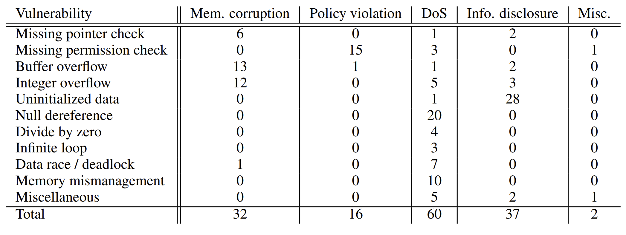
Denial of service (e.g., kernel crash) is the most common consequence, and is largely due to NULL pointer dereferences, and to a lesser extent to memory mismanagement (e.g., leaks).
Next come vulnerabilities allowing an attacker to read (information disclosure) or write (memory corruption) kernel memory.
Unsurprisingly, memory corruption issues are largely due to buffer and integer overflows.
Information disclosure is itself mostly due to the kernel sending uninitialised or partially initialised data through I/O channels or to user space: that uninitialised data may contain old kernel data, for example in the case where the kernel’s equivalent of malloc reuses freed memory without zeroing it.
A second table studies the location of these vulnerabilities in the kernel code base:
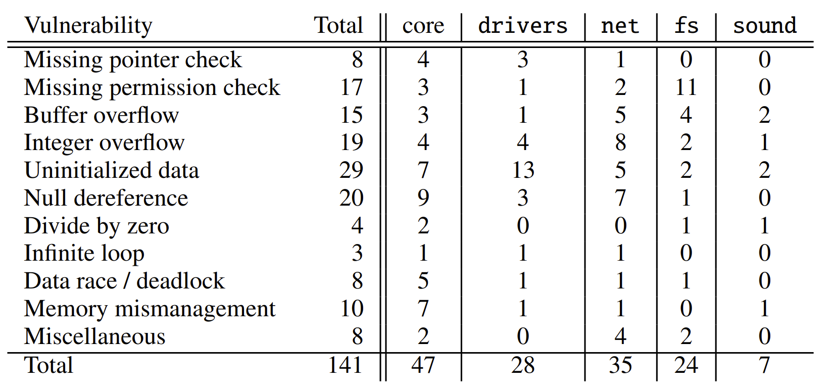
About a third of the vulnerabilities are located in the core kernel code, that is the part of the code included with every compilation of Linux. The other two thirds of the vulnerabilities are located in kernel modules: driver, networking, filesystem, and sound management code.
Linux: Runtime Defences
Linux offers a set of runtime defences, some specific to its OS nature, others similar to the protections we already covered for applications.
Attack Surface Reduction
Kernel Memory Permissions. Linux implements a strict memory access permission model for the kernel. The goal is to restrict memory permissions for the kernel as much as possible, while still letting the OS do its job properly. It is a direct application of the least-privilege principle. A key part of the relevant policies is that kernel executable code and read-only data must not be writable. The kernel code is particularly sensitive because it runs with supervisor privileges, so preventing it from being written as far as possible is important: this is the write xor execute protection we already covered for applications. Kernel function pointers and sensitive variables are similarly sensitive, and should not be easily writable.
Two memory protection technologies help further isolate the kernel from user space attacks:
- Supervisor Mode Execution Prevention (SMEP) prevents the kernel from executing code located in user-space memory.
- Supervisor Mode Access Prevention (SMAP) prevents the kernel from reading/writing user-space memory.
Both technologies are enabled on most modern CPUs and protect against injection and dereference of user space pointers in the kernel (ret2usr attack).
Note that user space can still indirectly control a subset of the physmap, a particular area of the kernel memory that is a direct mapping of all physical memory (that by desing include the memory allocated to user space processes).
Attacks leveraging that area are called ret2dir.
Note that SMAP must be temporarily disabled by the kernel during copy_to/from_user.
Reducing Applications’ Access to System Calls. Most applications make use of only a small subset of the system call interface exposed by Linux. Preventing an application from issuing the system calls it does not need to perform its job is called system call filtering:
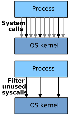
System call filtering is a common kernel protection measure against untrusted applications, as a subverted program attempting to attack the kernel may issue system calls it does not normally invoke under legitimate execution. This is widely used in production to harden multi-tenant and sensitive environments, such as Docker containers, Android or Flatpak/Appimage software, etc. This is achieved under Linux with a software technology named seccomp.
A particular problem with system call filtering is how to determine precise, per-application system call blacklists and whitelists? Determining a good black/whitelist manually for every application in a distribution requires a huge amount of effort, so automation is needed. However, automated techniques rely on either static or dynamic analysis, with each method coming with its own downside. Static analysis overestimates the legitimate system calls that can be issued by an application, which translates into filtering rules with low strictness. The coverage limitations of dynamic analysis raise the concern of missing system calls that may be legitimately invoked by an application but are not exercised during analysis, which may lead to legitimate system calls being flagged as an attack in production.
Probabilistic Defences
Similar to user space programs, stack canaries and ASLR are supported by the kernel. These probabilistic protection techniques come with the same pros and cons as for user applications. Canaries allow detecting certain attempts at overwriting return addresses on kernel stacks, however there is only a single canary value for all stack frames on each CPU core. Should this value leak to the attacker, e.g., through a stack buffer overread, the protection may be bypassed. The kernel also applies Address Space Layout Randomisation (KASLR for Kernel ASLR) to the kernel memory areas. Same as for user space it is coarse-grain in nature: upon creation, a random offset is added to large areas including kernel and modules executable code, kernel stacks, vmalloc area, physmap, etc. Because of that coarse granularity of randomisation, a single pointer leak may allow an attacker to break ASLR for the entire area.
Memory Integrity
Regarding control flow integrity, the Linux kernel supports Indirect Branch Tracking, a CPU technology that restricts the target of function pointer calls to a set of legitimate functions. Shadow stacks are not currently supported by the kernel.
To further protect against overflows, the kernel places guard pages at the beginning and end of kernel and user space stacks. Guard pages are unmapped pages that trigger a fault when accessed. Should a linear stack over/underflow escape the stack and hit one of the guard pages, the resulting fault would allow the issue to be detected:
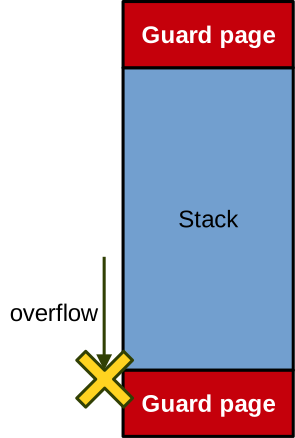
Other protection techniques include macros for arithmetic operations that embed overflow checks, and sanity checks applied to heap metadata to detect corruption during the dynamic allocation and deallocation of memory in the kernel.
Preventing Kernel InfoLeaks
Kernel information leaks happen when data supposed to be private to the kernel becomes inadvertently readable by untrusted security domains such as user space or remote applications. This may allow an attacker to steal sensitive data (e.g., passwords) or infer information about the kernel that may be useful to mount further attacks. A notorious example here are kernel pointers: as we have seen previously, kernel address space layout randomisation is applied on a coarse-grain basis, so having a single kernel pointer leak to user space may allow an attacker to break ASLR and infer part of the kernel memory layout, which is required for many attacks.
To avoid such issues, the kernel must take care not to send to user space buffer or data structures that are only partially initialised: because dynamic memory allocators generally reuse memory without zeroing it out (for performance reasons), such uninitialised memory may contain old kernel data. Although that old data has been freed, it can still be useful to an attacker, e.g., old kernel pointers can still allow to break ASLR. The kernel also takes care of not using addresses as resource identifiers, but rather numbered identifiers such as file descriptors.
A tempting solution to the issue of kernel leaks stemming from reusing dynamically-allocated memory would be to zero out any piece of memory freed with the kernel’s equivalent of free.
That way when the memory in question is reused and possibly leaked through a partially-initialised data structure or buffer, it does not contain any information of value to an attacker.
Unfortunately, this solution is generally too costly from a performance point of view: calls to free are often located on the critical path of performance-sensitive operations, and the amount of time required to zero out freed memory is often unacceptable.
Linux: Bug Detection
Similarly to applications, dynamic and static analysis techniques have been applied to the Linux kernel with the goal of detecting bugs and security vulnerabilities.
Dynamic Analysis Techniques
Several dynamic analysis techniques are applied to the Linux kernel for bug detection. Kernel sanitisers such as Kernel Address Sanitiser (KASan), Kernel Undefined Behaviour Sanitiser (KUBSan), as well as memory leaks and concurrency (race conditions) sanitisers are widely used to detect memory errors and undefined behaviour at runtime. Lockdep tracks the state of locks to detect deadlocks, double locking, and lock order inversion. Dynamic tracing and instrumentation tools such as ftrace, perf, and eBPF provide runtime observability into kernel behaviour. Finally, fuzzing tools can also be used to protect the interfaces exposed by the kernel to untrusted security domains. We have seen earlier that the system call interface represented a primary attack vector for the kernel, and understandably significant effort has been devoted to fuzzing it.
Syzkaller: Fuzzing the Linux System Call Interface. Syzkaller is a widely used kernel fuzzer targeting the system call interface. It works by injecting malformed system calls into kernel space with the hope of triggering bugs. The kernel under test is generally compiled with sanitisers enabled to maximise the chances of detecting bugs, and executed in a virtual machine. Fuzzing is controlled from the host: for each round of fuzzing a program containing a series of syscalls to execute is generated and executed in the VM. Syzkaller is a coverage-guided fuzzer, meaning that it measures the kernel code coverage executed by each injection of system calls, and uses that information to generate the next series of system calls to execute in a way that maximises the chances of hitting new coverage. Syzkaller fuzzing process is illustrated in the following diagram:
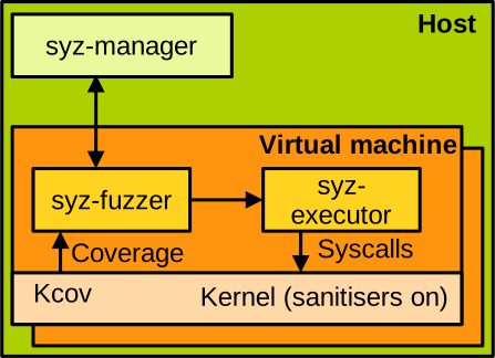
Syzkaller is a grammar-based fuzzer, meaning that the fuzzer models the interface it aims to fuzz, the Linux system call API, as a language.
That language is called the Syzlang, which is a grammar used to precisely describe the different system calls Linux supports, how they interact with each other, and the data flowing in and out of that interface.
The Syzlang models system calls arguments and their types, the data structures that can be passed between system calls (e.g., a file descriptor can be created by open and used later by read) for file I/O, the length parameter specifying the size of other parameters, etc.
This precise knowledge of the system call interface lets Syzkaller optimise the generation and mutation of fuzzing inputs, to maximise the chances of hitting new coverage and discovering bugs.
Below is an excerpt from the Syzlang:
resource fd[int32]: 0xffffffff, AT_FDCWD
resource sock[fd]
resource sock_unix[sock]

socket(...) sock
accept(fd sock, ...) sock
listen(fd sock, backlog int32)
On top of this snippet we can see examples of definitions of data structures flowing through the system call interface: a file descriptor fd is a signed integer on 32 bits, and can take the notable values 0xffffffff or AT_FDCWD.
A socket sock is a special type of file descriptor, and a Unix socket is a special type of socket.
Next come three examples of system calls.
The socket system call returns a socket.
The accept system call takes as first parameter a socket file descriptor, and returns another socket file descriptor.
Finally, the listen system call also takes a socket file descriptor as first parameter.
The Syzlang lets Syzkaller generate for fuzzing series of system calls that make sense together, for example, generate a socket file descriptor with socket and then pass it on to listen.
Syzkaller is widely used by Google to continuously fuzz Linux, Android, FreeBSD, NetBSD, OpenBSD, and gVisor, through a system called Syzbot. It consists in hundreds of VMs fuzzing these OSes 24/7. Thousands of bugs have been uncovered this way, and reported automatically to the OSes’ developers. The results are accessible online on Syzbot’s website. The graph below is taken from that website, and represents the number of bugs discovered (red line) and fixed (green line):
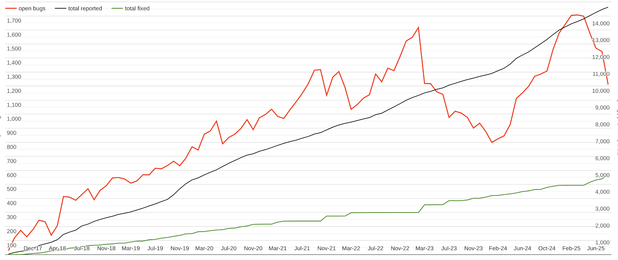
As one can observe, there is an important amount (two thirds) of invalid bugs reported. There are multiple reasons for a bug to be classified as invalid: secondary symptom of an earlier memory corruption, duplicate of another bug, etc.
The Linux Test Project. The Linux Test Project is a repository of test cases maintained by a series of companies and institutions outside of the kernel main tree. It contains many tests targeting various subsystems of Linux: system calls, conformance to the POSIX standard, filesystems, networking, memory management, etc. It also contains test cases reproducing existing kernel CVEs.
Static Analysis Techniques
Several approaches also apply static analysis to the problem of bug detection in the Linux kernel.
Pattern-based analysis tools such as Coccinelle and Smatch allow developers to describe common programming mistake patterns in source code.
For example, a pattern can specify that for every call to kmalloc there should be a corresponding kfree, enabling automated detection of memory leaks.
Control and data flow analysis tools like Sparse let the programmer use compiler attributes to annotate certain properties on objects and memory.
For instance, the __user attribute can mark pointers that reference user-space memory (used for example in copy_to/from_user, see above), while __acquires can indicate a lock that is held on function exit but not on entry, helping to detect incorrect locking patterns.
Other approaches include formal verification techniques, symbolic execution, and various compiler-based analysis methods.
Similarly to applications, a key challenge for kernel static analysis approaches is their inherent scalability issues, particularly around state explosion. These downsides are particularly problematic when applied to OS kernels, because of the sheer size of their code bases, that are often in the order of millions of lines of code.
OS Security Concepts Part 2
You can access the slides 🖼️ for this lecture.
We have seen in the previous lecture how the kernel protects itself against external threats. Here, we discuss how the kernel exposes access control mechanisms to user space to protect various resources.
UNIX/Linux File Permissions
Linux is a multi-user operating system: several users that do not trust each other share the same machine. There is also at least one privileged system administrator, often named root, that does not trust the regular users. Hence, the OS must make sure the files and system resources are properly isolated to respect that trust model.
Linux is heavily inspired by UNIX and in particular it follows one of its main principles which states that everything is a file. Beyond regular files, this also applies to devices, IPCs, OS metadata and configuration knobs, among others. As a result, many security mechanisms that define what users and processes can and cannot do rely on file permissions. These permissions not only let users and applications access files (or not), but also devices (e.g., camera or microphone), OS functionalities (shutting down the computer, installing new software, etc.) and information (kernel log, etc.), etc.
You probably already have a certain amount of knowledge about file permissions. Here we have an example of such permissions in the form of an access control matrix, a concept defined by Lampson in his seminal paper, Protection:
| File A | File B | File C | |
|---|---|---|---|
| Process 1 (user 1) | read, write | read | - |
| Process 2 (user 2) | read | write | read |
In the first column you have what is called subjects; here they are processes, but they could also be users. In the first row we have objects; these are files that subjects may or may not access. Finally in the rest of the matrix, at the intersection between a subject and an object, you have the list of permissions that subject has upon that object. For example, here process 1 can read and write file A, can read file B, and cannot access file C at all. Process 2 has different permissions: it can read file A, write to file B, and read file C.
Each process running in the system is associated with a user ID, and a group ID. In the vast majority of cases, when a user invokes a program, the process will take the user’s UID and GID. Each file in the system is associated with an owner user ID and owner group ID. So given a particular file, processes executing with a UID equal to the file’s owner UID can change permissions on that file; in other words, they have full read/write/execute permissions. Processes executing with a GID equal to the file’s owner GID can also obtain additional permissions compared to processes running with unrelated UIDs and GIDs. The permissions are defined within each file’s metadata on the filesystem: there are specific bits for that, named the permission bits.
We can check a process’ UID and GID by using the ps command as follows:
# Check a process' UID/GID
$ ps -o pid,user,group,uid,gid,comm -p <pid>
We can also review a file’s owner UID and GID, as well as the value of its permission bits, with the ls -ln command:
# Check a file's UID/GID and permission bits
$ ls -ln <file>
Listing a file’s permissions and owner UID and GID with ls gives you the following output:
$ ls -l /usr/bin/cp
-rwxr-xr-x 1 0 0 151152 Sep 20  2022 /usr/bin/cp
The string with dashes and the r/w/x characters, -rwxr-xr-x, gives us the file type and permissions; we’ll zoom in on that information shortly.
The first 1 after that is the number of hard links to the file.
The next two zeros 0 0 coming next are respectively the file’s owner UID and GID.
The number coming next, 151152, is the file size in bytes.
The rest of the information is a timestamp for the file’s last modification Sep 20 2022, and the file path on the filesystem /usr/bin/cp.
Let us focus a bit on the permissions string reported by ls:
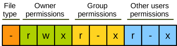
The first character represents the file type.
It’s a dash - for regular files, a d for directories, and you’ll find other characters for special files representing things like devices or IPC channels.
Then we have three blocks of three characters each, representing permissions for subjects.
The first three characters give the permissions for the file’s owner UID, the second set of three characters gives the permissions for the file’s owner GID, and the last three characters give the permissions for anyone else.
The permissions can be read access, permitted with an r and prohibited with a dash; write access, permitted with a w and prohibited with a dash; and execute permission, for executable programs, enabled with an x and prohibited with a dash.
Here is an example of how the permissions could be set up on a university lab machine that is shared between students and faculty:
| Name | Owner | Group | Mode bits |
|---|---|---|---|
foo | alice | faculty | rwxr--r-- |
bar | bob | students | rw-rw-r-- |
baz | charlie | faculty | rwxrwxrwx |
Users are classified into groups, students and faculty, and each file has a user owner, as well as a group owner.
foo is accessible with full permissions by Alice, but can only be read by the faculty group and other users.
bar is readable and writable by Bob and by anyone from the students group; it can only be read by other users.
Finally, baz is fully accessible by anyone.
Authorisation Mechanisms
System administrators use user space applications to configure permissions for files.
An authorised user can change the owner of a file with chown, and the file’s permissions with chmod.
When files are accessed, the permission checks are performed by the kernel upon each access, with the relevant system calls: open, read, write, etc.
When a user authenticates, the authentication program, like login or ssh, needs to run as root, which means it has system administrator privileges.
This is because, if the authentication succeeds, the process needs to switch to the identity of the authenticated user, and the ability to switch identity is a privileged operation that should not be possible for a standard user.
After that identity switch, all subsequent processes will inherit the user’s identity.
The system also integrates programs providing some services that are supposed to be invoked by standard users but that require root privileges.
An example is the passwd command, which users can invoke to change their password.
This program needs to update the central system password file /etc/shadow, which obviously cannot be accessed by normal users, only by root.
So passwd has a special permission bit named the setuid flag, which lets it be invoked by a standard user while actually running with root privileges.
This has important security considerations, which we will cover in more detail in the second lab exercise.
Discretionary Access Control
As we saw, with traditional UNIX file permissions, non-administrator users can change the security configuration of the system because they manage the permissions for their own files.
They do so by updating permission bits and owner UID/GID for the files they own, for example with chmod.
A system in which regular users can update security permissions is called Discretionary Access Control, DAC.
DAC is not ideal from a security point of view, as it assumes that users are fully trusted and that they always behave correctly.
This is not the case in reality.
First, users can make mistakes: imagine a user A executing a wrong chmod command, mistakenly allowing other users to access their private files, for example a private SSH key.
Second, some users or processes can also be actively malicious.
Imagine a remote attacker taking over a user process’s execution flow by exploiting a use-after-free vulnerability.
That attacker could manipulate the program to lower the defences of the system, by changing its security configuration through file permissions.
So, unfortunately, the assumptions behind discretionary access control do not hold in reality, and DAC is not a very secure solution.
We need a protection system that maintains security guarantees even when software outside the trusted computing base is malicious.
Mandatory Access Control
Mandatory Access Control (MAC) addresses the aforementioned problem: with MAC, the security configuration can only be modified by trusted administrators. Every subject (process) and object (file, system resource) receives a security label. Labels are used to define rules describing how processes can interact with each other and with system resources. The set of labels is defined by the trusted administrator, and labels are assigned to processes and objects at creation time. At runtime, the security policy is immutable: trusted software can be used by administrators to update it, but restarting the protection system is needed for the changes to take effect, and this can also only be done by an administrator.
Below is an example of a mandatory access control policy, adapted from the book Operating System Security by Trent Jaeger:
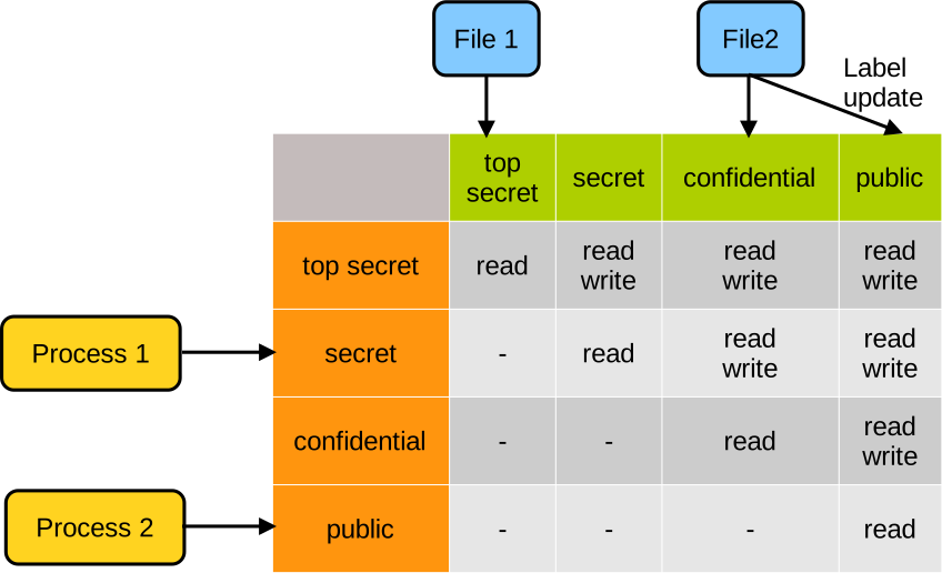
We have our subjects on the left, two processes. Process 1 gets assigned the secret label when it is created. And process 2 gets assigned the public label. On top we have our objects, two files. File 1 gets assigned the top secret label, and file 2 gets initially assigned the confidential label. Note that subject and object labels do not necessarily have to be the same. Within the matrix you can see the permissions: process 1 being secret, it cannot access top secret files like file 1, and can read and write confidential files like file 2. Process 2 being public, it can access neither file 1 nor file 2. If the administrator wants to change the labelling, that would require a restart of the MAC system. For example here file 2 becomes public and can then be read by process 2.
SELinux
Linux has a mandatory access control framework named Security Enhanced Linux (SELinux).
With SELinux, processes, files and system resources get assigned labels that are called contexts.
A context has, among other attributes, a type.
A few examples of context types are httpd_t for a running web server, httpd_sys_content_t for content being served by that server in /var/www/html on the filesystem, or http_port_t for the port the server is listening on.
As defined by the MAC working principles, the security policy is defined by a trusted administrator. Rules explicitly describe the possible operations processes can perform on files and OS resources. For example, our web server will get access to both the files it needs to serve and the ports it needs to listen on. When an action is performed, SELinux checks are done after the traditional filesystem permission checks. Note that, with SELinux, no rule means deny by default, so the policies are quite strict; when they are well-defined, they represent a good way to achieve least privilege for the system.
Below is an example of SELinux policy for 2 processes here, a web server and an SQL database:
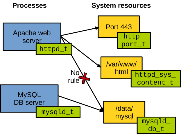
Each process is labelled with its own type. The web server can access the usual port serving HTTPS requests, as well as the files it is supposed to serve on the filesystem. The SQL database gets access to the filesystem location where the database is stored. Because there is no rule allowing it, the web server cannot access the database file. The database also cannot access the web server’s port or the files it serves.
SELinux: Benefits and Limitations. As we saw, MAC implemented with SELinux is very strict and is a good way to enforce least privilege on a fine-grained basis. For example, if the web server is compromised by an attacker, the attacker will only be able to access whatever SELinux allows the web server to access. With traditional file permissions the attacker would get access to many more system resources. If the web server was running as root, which would be terrible from a security point of view, the attacker would gain full access to the entire machine. Even if the server was not running as root, the attacker would still get access to everything the user it runs on behalf of can access. Another benefit of SELinux is that it is widely available, and required for certain compliance standards.
Unfortunately, there are also some downsides to using SELinux. The main issue is that it is difficult to configure, manage, and troubleshoot. Many actors really struggle with it, just Google “how to disable SELinux” to get an idea. It is also sometimes too strict, so it creates some false positives at runtime, flagging legitimate behaviour as security issues.
Linux Security Modules
SELinux is mostly concerned about the rules defining what processes and users can do with which files and system resources. A specific set of such rules represents what is called a policy. To enforce these rules we need a mechanism that will hook into file and resource accesses, and will deny or approve these accesses based on what is defined in the policy. With Linux this mechanism is called Linux Security Modules (LSM). It is a mechanism framework on top of which many access control systems are built, SELinux but also systems like Smack, TOMOYO Linux, or Apparmor:
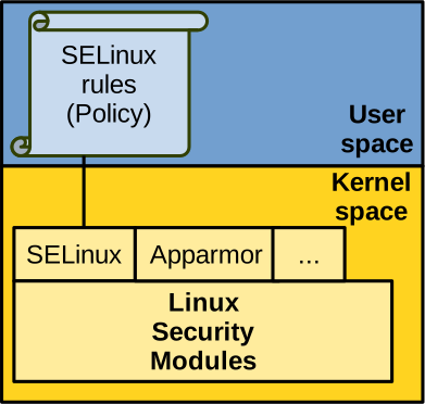
From a high-level point of view, LSM works as follows.
LSM uses hooks on the relevant kernel code paths, at the point the kernel accesses security-critical resources, for example at the time a file is opened.
The security modules in place, for example SELinux, can then permit, deny, and/or log operations for auditing.
Many kernel data structures have a generic void * pointer named security that can be used to hold any kind of relevant security metadata.
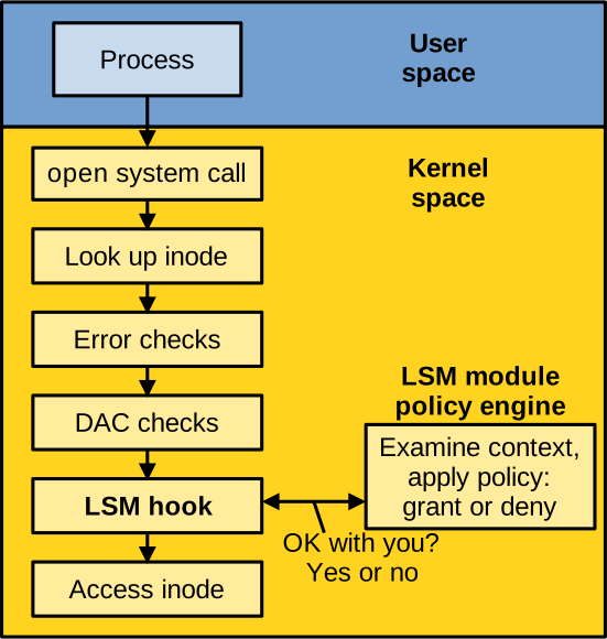
You have an example on the diagram above (adapted from Wright et al., Linux Security Modules: General Security Support for the Linux Kernel): when a process opens a file the kernel starts to process the system calls, and looks up the inode for the file in question. The kernel performs some basic error checks (for example, does the file exist?), then performs the discretionary access control checks first on traditional UNIX file permissions. Next, we have the LSM hook, plugged to the policy in place, that could be for example SELinux. Whatever handler is called there will allow, deny or log the operation. If the operation is allowed, it can then be performed.
Capability Systems
The Confused Deputy Problem
Access control systems are not very efficient in all situations. Here is a classical computer security problem called the confused deputy, which access control systems do not handle well. It has been described in the following paper: Norm Hardy, The Confused Deputy (or why capabilities might have been invented).
Imagine a shared, multi-user system used to compile some code.
Users have a home folder /home/user with their source code src.c.
They invoke the compiler, passing the source file as a parameter, as well as the name of the executable they wish to create, a.out.
They can also dump debug symbols into a separate file, here named debug-info.
The system administrator has also configured the compiler to write down a summary of language usage statistics in a file located within a system directory: /sysx/language-stats.txt:
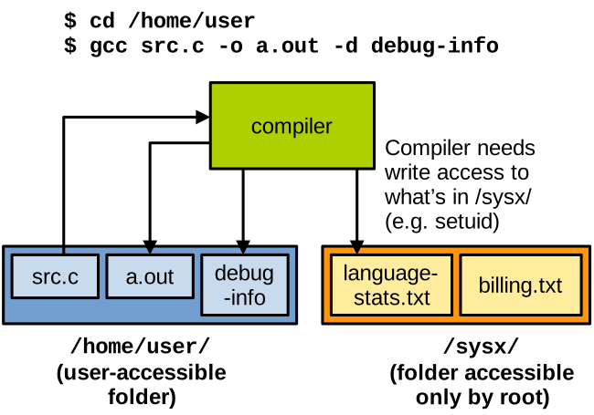
That system folder /sysx/ is supposed to be accessed only by root; however, because the compiler needs to write to it when invoked by the user, the administrator configures the access control system to let the compiler program write to that folder to dump the language usage statistics.
In /sysx there is also a sensitive file that contains some important billing information, billing.txt.
This file should not be accessible to normal users.
If a user somehow learns about the existence of the sensitive file billing.txt, for example by discussing with a colleague, they can trick the compiler into overwriting that file.
For example, by indicating it as the target for writing the debug symbols, as presented here:
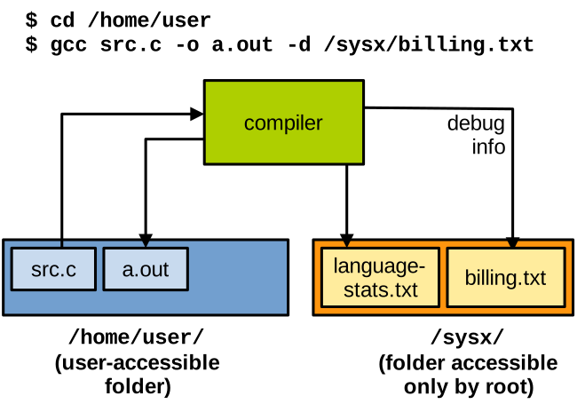
So in effect we have a subject with a certain amount of privilege, which we name a deputy (here the compiler), confused into accessing a resource that the user it runs on behalf of does not have permission to access.
Capability Systems
There is no good way to solve the confused deputy problem with access control systems (DAC/MAC), because they do not make it possible to have the deputy (the compiler) execute with the permissions of the user invoking it: the compiler needs to run with its own permissions, which need to include access to the sensitive folder.
To address that issue, a different approach can be used: capability systems. A capability is a token that can be held by a subject, and that brings together:
- The ability to designate a resource, for example the ability to name a file or reference a particular device; and
- The permissions to access that resource.
In other words, with capabilities, if you can name a resource, you can access it.
This differs from access control systems, where you can name resources that you can’t access: for example, as a standard user you can ls /etc/shadow although you can’t access it.
Capabilities can also embed specific access permissions: e.g., a capability may allow a user to access a file in read-only mode, and another capability would allow another user to access that file in write mode.
In capability systems, subjects (processes, users) are called principals. Each principal is given a set of capabilities corresponding to the system resources (files, memory, CPU time/cycles, ports, devices, etc.) it is authorised to access. The operating system has ambient authority, i.e., it can access all capabilities. Principals that interact with each other can exchange capabilities as a form of permission delegation. For example, a parent process can give a subset of its capabilities to a child process it forks. In another example, process A can give access to part of its address space to process B with which it wishes to establish shared memory-based inter-process communication.
Principals cannot forge capabilities out of thin air, and the only way for a subject to obtain a capability is to receive it through the aforementioned delegation process. Principals can only make copies of capabilities they already have access to, and such a copy can only have similar or lower permissions compared to the original capability it is based upon. In other words, it is not possible for a principal to forge a capability out of thin air. This is a key property of capability systems, called monotonicity.
After the OS boots, it has access to all the capabilities and can access all resources in the system.
The OS then creates the first process, let’s call it init, giving it a subset of the system’s capabilities.
init creates other processes, granting each a subset of its own capabilities based on what each process needs.
Sets of capabilities continue to be subset from parents to children.
Because processes cannot forge capabilities, there is no way for them to increase the permissions that were given by their parents.
Solving the Confused Deputy Problem with Capabilities
This diagram illustrates how capabilities can help solve the confused deputy problem:
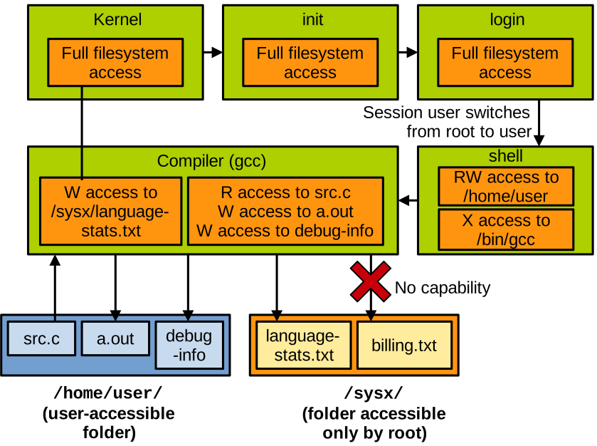
For the sake of simplicity we will only consider capabilities relating to file access.
When the OS boots up, it is initialised with all the capabilities, meaning it has access to the entire filesystem.
It creates the first process init which itself creates login, both of these run as root because the user is not authenticated yet, and they both get a copy of the entire set of capabilities letting them access the entire filesystem.
Once login has authenticated the user, it spawns a shell.
This shell will run on behalf of the user, so login subsets its capabilities for the shell based only on what the user is supposed to legitimately access.
In our example it is read/write access to the content of the user’s home directory /home/user, and execute access to the compiler /bin/gcc.
When the user runs the compiler, the shell subsets its capabilities again and gives the compiler only what it needs: read/write access to the source file src.c, the executable output a.out, and the debug symbols output debug-info.
The compiler also requires a write capability to /sysx/language-stats.txt.
It could be passed down the capability subsetting chain; however, that would let other principals, like the shell, access the file in question, which is not really needed.
That capability can instead be obtained by the compiler from the kernel, which has full access to the filesystem.
In that context, our aforementioned confused deputy problem cannot happen: when it executes on behalf of the user, the compiler cannot have a capability to access the billing file, and won’t be able to overwrite it.
Trusted Execution Environments
You can access the slides 🖼️ for this lecture.
This is a brief introduction to Trusted Execution Environments. These represent hardware-assisted isolated computing environments, which enforce a specific trust model that is particularly strong.
Introduction
Imagine a server owned by a cloud provider, sitting in a data center and used for cloud computing. This cloud provider executes several virtual machines on top of that server, and each of these machines is rented to a different client. In the context of cloud computing, these clients are named tenants.
Let us reason about the different trust models at play in that scenario. From the cloud provider’s point of view, the hardware is trusted, so is the privileged software handling the virtualisation: that is the virtual machine monitor, some host-level software, and so on. What the cloud provider does not trust is: everything run by tenants within the virtual machines, i.e., tenants’ applications and guest operating systems. The cloud provider has no idea what the tenants will run in their VMs, and needs to assume that software may be malicious.
If we now take the point of view of one of the tenants, they trust their own software. Tenants also trust the cloud provider’s hardware and software such as the virtual machine monitor. Finally, tenants distrust each other: processes running on the same OS, we don’t want a VM belonging to one tenant accessing the memory of a VM belonging to another tenant.
Trusted Execution Environments (TEEs) target the enforcement of a stronger trust model. They still consider that the cloud provider distrusts tenants and that tenants distrust each other. But there is an additional component: tenants do not trust the cloud provider. This makes sense today: a lot of companies are reluctant to move their workloads to the cloud because they don’t want the big cloud providers to get access to their code and data. In that context, the objective of TEEs is to create an isolated execution environment and maintain confidentiality and integrity for software executing in it, in the presence of untrusted privileged software. Here, untrusted privileged software concretely means that we consider a VM that does not trust the hypervisor managing it, or a process that does not trust the operating system it runs on top of. In our cloud scenario, the distrust relationships between provider and tenants can then be illustrated as follows:
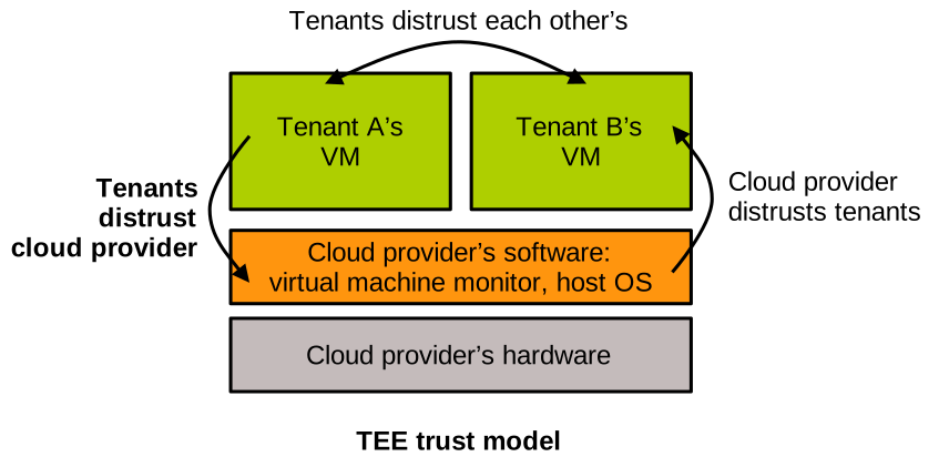
What is a TEE?
A TEE is a hardware-enforced isolated execution context in the CPU. The isolation is strong enough so that the privileged layers, namely the OS or the hypervisor, can neither read nor write within that environment. Because they protect against read and write accesses, TEEs enforce confidentiality and integrity. They cannot really enforce availability: that is too difficult in the presence of an attacker strong enough to run privileged software. For example, because the attacker can run OS code in supervisor mode on the CPU, nothing prevents them from simply shutting down the machine to affect availability. A classic TEE threat model assumes attackers may control: all host software outside the TEE, including privileged layers such as the OS or hypervisor, as well as I/O devices.
Key Characteristics
We are going to see next three different implementations of trusted execution environments. They all share the following key characteristics. First, as previously mentioned, they all enforce strong isolation for the software running within the TEE, through some form of isolation mechanism. The outside world, including the privileged software like the OS, cannot read or write the memory allocated to the TEE. Second, this isolation implies controlled interactions between the TEE and the outside world. Indeed, a TEE is not entirely self-sufficient and needs to interact with the OS or the hypervisor to perform I/O. These interactions need to be secured as, contrary to traditional trust models, the OS and the hypervisor are not trusted by the TEE.
TEEs also provide some secure storage for sensitive data such as cryptographic keys or passwords. That secure storage is itself realised with encryption keys that never leave the TEE. Finally, because most TEEs are accessed by their users remotely, such remote users need a guarantee that:
- The TEE they connect to runs on the right hardware, i.e., a CPU with support for trusted execution environments; and
- The untrusted owner of that hardware has loaded the right software within the TEE, not a version that has been tampered with, e.g., to confuse the user into entering sensitive data.
Obtaining such guarantees is possible through a mechanism called attestation. We will cover it in more detail toward the end of this lecture.
Use Cases
TEEs are useful in many scenarios. We mentioned cloud computing, where the cloud provider may not be trusted. They also play a key role for secure data storage applications, such as password managers, or personal data storage software, for example applications storing fingerprints or other biometric data on smartphones. More generally, TEEs are useful in scenarios where trusted code needs to run and process trusted data in hostile environments, where the rest of the system is almost entirely untrusted: DRM systems, confidential data processing such as ML training/inference, healthcare applications, and so on.
TEE Implementations
Next, we cover the main TEE implementations available from the principal CPU designers: Intel, AMD, and ARM.
Intel Software Guard Extensions (SGX)
One of the earliest implementations of TEEs was made by Intel, and it is named Software Guard Extensions (SGX). SGX places the trusted code and data in user space within what is called an enclave. At any time, the CPU runs either within or outside of the enclave. The enclave’s memory pages are encrypted and cannot be accessed from outside. Memory decryption is done transparently when the CPU runs within the enclave. A traditional SGX setup is illustrated on the left-hand side of this diagram:
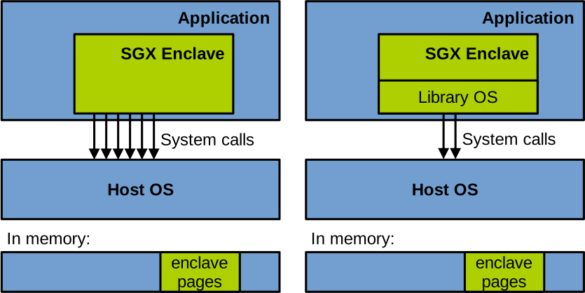
The enclave still needs to go through the untrusted host OS if it wants to perform system calls, for example for I/O. This requires transitions outside the enclave, something that is not only slow, but also represents an attack vector, because according to the threat model of TEEs, the OS could be malicious and return corrupted information. Hence, most of the frameworks that help develop enclave applications will embed within the enclave a small operating system, called a library OS (LibOS), which aims to process as many system calls as possible within the enclave, avoiding some of the costly and dangerous enclave exits. This is illustrated on the right-hand side of the diagram above. Even with a LibOS, for disk and network I/O, the untrusted host OS still needs to be invoked.
AMD Secure Encrypted Virtualisation
A particular issue with Intel SGX is that existing applications need to be modified to run as enclaves:
- They need to be adapted to connect to an enclave framework that generally includes a small library OS.
- Within the enclave, the data returned by I/O system calls also needs to be sanity-checked, because it comes from the untrusted host OS.
This is a significant downside, because very few developers would be ready to maintain a specific branch of their application for compatibility with SGX. AMD’s TEE implementation is called Secure Encrypted Virtualisation (SEV), and attempts to address that compatibility issue. SEV places an entire virtual machine, called a confidential VM, within the TEE. The entire VM’s memory is isolated and encrypted, similarly to what SGX does for an enclave’s memory:
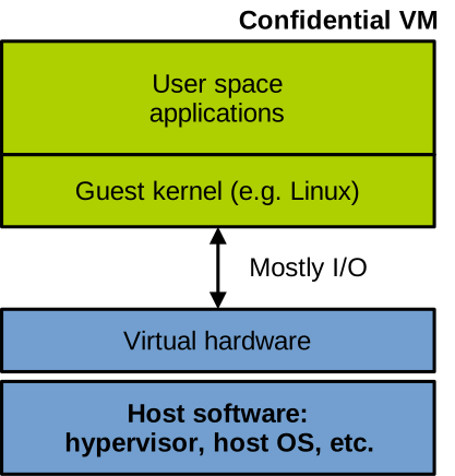
The advantage with SEV is that existing applications do not need to be ported; they can run as is. The main drawbacks are twofold. First, a confidential VM integrates a large trusted computing base, which includes the application but also the entire guest operating system. Second, for I/O, the VM still needs to go through the untrusted hypervisor, and that interface has proven very hard to secure.
ARM TrustZone
ARM’s implementation of TEEs is called TrustZone. With TrustZone, the CPU execution mode is dissociated between the normal world (outside the TEE), and the secure world (the TEE). These modes are orthogonal to privilege levels like supervisor or user modes, which are available in both normal and secure worlds. Once again, the hardware prevents the normal world from accessing the memory allocated for the secure world – although this time there is no memory encryption.
In the secure world, a small, secure OS runs, on top of which trusted applications running user code can execute. In the normal world, regular applications can invoke trusted applications:
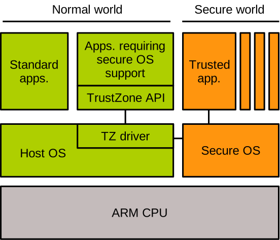
For example, if you are running Android and use your fingerprint to unlock your screen to access your bank or NHS app, the app in question will invoke the fingerprint check trusted application within a TrustZone environment to verify your identity. This way, even if your phone gets stolen and the thief manages to root it, it is still very difficult to steal your fingerprints.
Remote Attestation
As discussed earlier, in a scenario where a client connects remotely to a TEE application that itself runs on an untrusted host, the client needs to make sure that 1) the application runs in a TEE on the expected hardware (e.g., an SGX enclave on a genuine SGX CPU) and 2) the application in the TEE is the expected one, and it has not been tampered with before being loaded.
This is achieved with a technique called remote attestation. The TEE sends the client some form of measurement (e.g., hashes) uniquely identifying the software running in the TEE and the hardware it executes upon. For example, with Intel SGX, a measurement of the enclave’s initial state is sent to the client. That measurement mostly identifies the enclave’s memory content at load time. This allows the client to certify that the application loaded in the enclave is the expected one. Intel also offers an attestation service that will validate the hardware:
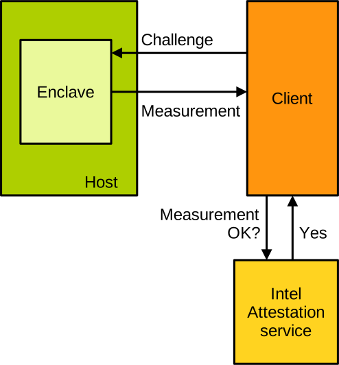
OS Models and Security
You can access the slides 🖼️ for this lecture.
OS Design Models
Since the first OSes were proposed in the 1950s, we have derived several classes of OS design models, coming from both industry and academia. Here, by OS design model we mean a collection of core design choices that define how the OS architecture is organised. Each of the main OS design models relevant today has pros and cons in terms of speed, memory footprint, reliability, real-time capabilities, and, of course, security. In this lecture we will briefly cover the OS design models that are relevant to security, and discuss their performance and security implications.
Monolithic Kernel
The monolithic kernel is one of the most widespread classes of OS design today. This is the model we focused on in this unit, as Linux is indeed a monolithic kernel. The key idea of a monolithic kernel is that all kernel components are packed together within a single trust domain: there is no isolation between kernel subsystems, and they all live within the same address space. Further, the kernel is closely coupled with applications, as both are located within the same address space: The OS is isolated from applications using CPU privilege levels: the kernel runs in supervisor mode, and the kernel’s memory is protected with the supervisor bit in page table entries. Applications are isolated from each other by running in different address spaces. We can illustrate the monolithic kernel model as follows:
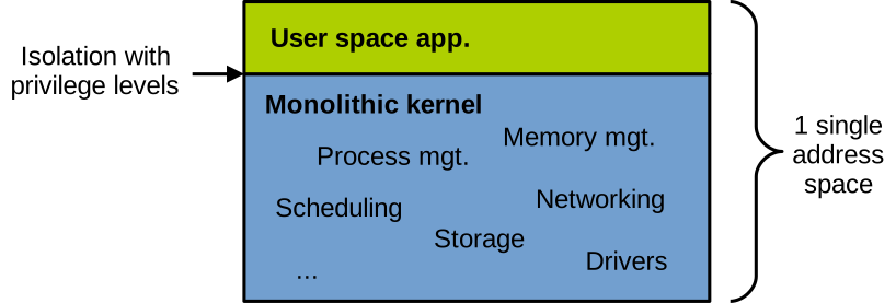
The close coupling of kernel and user space software components in a monolithic kernel is done for performance reasons, to lower the overheads due to the interactions between these components. Overall, this OS model gives us a middle-ground trade-off between security and performance. From the security point of view, the isolation between the kernel and applications, and between applications themselves, is good but not ideal, as we will see next. There is also no isolation inside the kernel. This medium level of isolation means that there is a limited number of security domain crossings, which is good for performance. Many derivatives of UNIX are monolithic, the most popular examples being Linux, FreeBSD, NetBSD, or OpenBSD. MS-DOS is another example of a monolithic kernel.
The OS Design Space
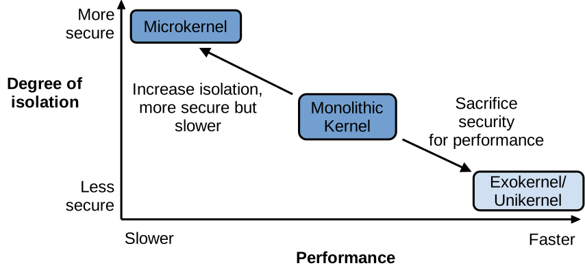
As we just mentioned, the monolithic kernel design is a middle-ground solution between security and performance. Let’s have a look at other, more extreme points in that design space. We can decide to increase the degree of isolation, to improve security at the cost of performance. We can also decide to sacrifice security for the sake of performance, for example by dropping part or all of the isolation between kernel components and/or applications, with the goal of faster computations.
Microkernels are a prime example of the former solution, favouring security at the expense of performance.
Microkernels
With a microkernel, most of the OS functionalities are moved into user space processes (sometimes named servers), each running within its own address space. The microkernel itself is very small and contains only the core functionalities that cannot be offloaded to user space: memory management, scheduling, as well as inter-process communication. These IPC mechanisms are a key aspect of microkernels, because this is the way used by kernel subsystems offloaded to user space to communicate with the rest of the OS.

The microkernel is considered more secure compared to the monolithic kernel, because of the increased level of isolation between kernel components. If one server gets compromised, the attacker will be confined to the relevant address space, and it will be difficult for them to gain access to the rest of the system. Of course, this additional security comes with a performance cost: communicating via IPC is slower compared to a monolithic kernel where everything lives within a single address space. With a microkernel, although the communication can be heavily optimised, such communication does involve security domain crossings and possibly data copies, all of which is expensive. Examples of microkernels include MINIX v3 and L4.
Exokernel
We now move to the other side of the spectrum presented earlier, looking at solutions that drop some or all of the isolation in the system to be able to run faster. With the exokernel model, each application or group of applications is compiled with a library providing most of the operating system services. This is called a library operating system (already briefly discussed in the previous lecture). LibOS instances run on top of a microkernel-like kernel named the exokernel:
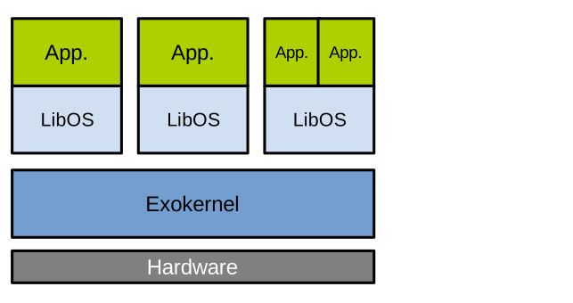
The exokernel acts as a microkernel, handling mostly core OS functionalities such as memory management, and exposing a low-level interface that securely multiplexes the hardware between the (untrusted) LibOSes. In its original version, the exokernel idea was to specialise each LibOS instance for the applications it runs, to maximise performance. Some applications could benefit from a particular implementation of the memory allocator, while other applications would prefer different implementations of the allocator. This is possible because we have one LibOS instance per application.
Unikernel
The exokernel idea was proposed in the 1990s but did not really take off. Fast forward to the 2010s, researchers realised that a small hypervisor could very well play the role of the exokernel, and that applications could be compiled with small library operating systems and run within virtual machines on top of that hypervisor. This is the unikernel design model:
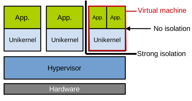
In terms of security, unikernels are well isolated from each other because they run in separate VMs. The hypervisor is also isolated from the unikernels. Still, there is no isolation between a unikernel instance and the applications it runs. This has some performance advantages, in particular system calls become function calls which are much faster. However, it is obviously concerning from the security point of view: if an attacker can exploit a vulnerability in an application, they may easily access the entire unikernel instance.
Operating Systems Part 2: Further Readings
Linux: Disk, Network, and Other I/Os
- Fischer, Linux Storage Stack Diagram. A much more detailed overview of the components of the Linux storage stack.
- (book) Love, Linux Kernel Development. Old but still relevant, check out chapters 13-16.
- (book) Bovet and Cesati, Understanding the Linux Kernel. Check out chapters from “The Virtual Filesystem” up to “The ext3 Filesystem”.
- Mathur et al., The new ext4 filesystem: current status and future plans. Describes the ext4 filesystem’s design (ext4 is the default concrete root filesystem in most Linux distribution).
- (book) Benvenuti, Understanding Linux Network Internals.
- (book) Corbet et al., Linux Device Drivers.
OS Security Concepts
- Chen et al., Linux Kernel Vulnerabilities: State-of-the-Art Defenses and Open Problems.
- Wang et. al., How Double-Fetch Situations turn into Double Fetch Vulnerabilities: A Study of Double Fetches in the Linux Kernel.
- Kemerlis et al., kGuard: Lightweight Kernel Protection against Return-to-user Attacks.
- Kemerlis et al., ret2dir: Rethinking Kernel Isolation.
- Hardy, The Confused Deputy: (or why capabilities might have been invented).
- Linux Test Project Contributors, Linux Test Project’s GitHub repository.
- Google, Syzkaller’s GitHub repository.
- (book) Jaeger, Operating System Security.
- Anderson, Security Engineering. Chapters available for free in PDF here.
Trusted Execution Environments
- Georgia Tech’s SSLAB, SGX 101.
- Confidential Computing Consortium, A Technical Analysis of Confidential Computing.
- ARM documentation, Learn the architecture - TrustZone for AArch64.
OS Models and Security
- Herder et al., MINIX 3: A highly reliable, self-repairing operating system.
- Biggs et al., The Jury Is In: Monolithic OS Design Is Flawed, Microkernel-based Designs Improve Security.
- Engler et al., Exokernel: An operating system architecture for application-level resource management.
- Madhavapeddy et al., Unikernels: Library Operating Systems for the Cloud.
Software Compartmentalisation: Introduction
You can access the slides 🖼️ for this lecture.
In this lecture, we introduce a defensive software design technique that has been used since the early 2000s to protect sensitive systems software, and that has recently gained renewed attention in research: software compartmentalisation.
Systems Software Security Landscape
Most systems software today is seen as a single, monolithic unit of trust. Concretely, this means that if an application (or operating system, hypervisor, library, etc.) has a single vulnerability anywhere in its code base, that vulnerability may allow an attacker to take over the entire application. That is because there is no internal isolation within the application in question. This is very concerning today. Indeed, modern applications integrate components from various sources with different degrees of trust:
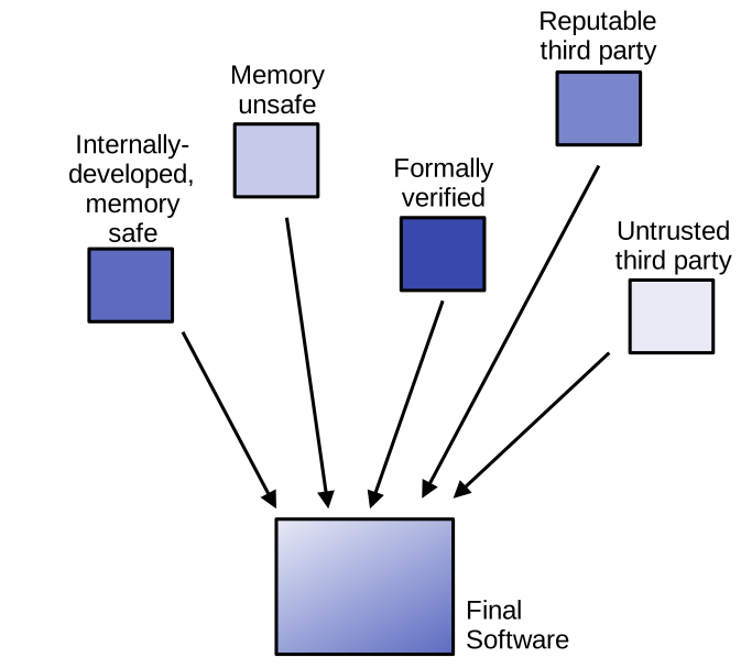
If we consider for example an application that links together several libraries, some of these libraries may have a high degree of trust because they are developed by a reputable third party, or because their correctness can be formally verified. On the other hand, other libraries may be less trusted, because they are developed by untrusted third parties, written in memory-unsafe languages, etc. The code of some libraries can also be under the control of an attacker, as shown in recent examples of supply chain attacks.
In addition to components with variable degrees of trust, systems software also integrates components that are security-critical: code handling secret data (passwords, crypto keys, etc.), performing privileged operations (user authentication, administrative tasks, etc.), etc. Mixing such sensitive software in an application without any form of internal isolation is very concerning from the security point of view. A natural conclusion from that problem statement is that we need to bring isolation and privilege reduction within applications. This can be achieved with a defensive software design technique called software compartmentalisation.
Software Compartmentalisation
Software compartmentalisation decomposes software into lesser-privileged components (compartments) that only have access to what they need to do their job. This approach is different from many other defences: with compartmentalisation, we acknowledge there will be bugs and exploits, and try to limit their impact. This is a direct application to software components of the principle of least privilege.
Let us take a concrete example, illustrated below:
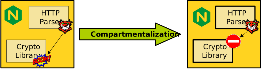
Assume a web server containing several software components and in particular:
- An HTTP parser: this code processes HTTP requests coming from the outside world. Parsers are complex pieces of software that are prone to bugs. Requests could also come from malicious actors and be malformed with the hope of triggering bugs in the parser. In the web server, the HTTP parser has a low degree of trust.
- A crypto library, such as libSSL. It handles HTTPS content encryption and decryption using security-sensitive data (e.g., crypto keys) that we do not want an attacker to get access to. In our example, the crypto library is critical to the security of the application.
Without any form of isolation between the two components, an attacker may exploit a bug in the parser to take over or leak data from the crypto library, which is catastrophic from the security point of view. Software compartmentalisation introduces some isolation between the two components, for example by placing the parser and the crypto library within separate compartments. An attacker triggering a bug in the HTTP parser would be unable to escape the isolation in question and access the crypto library.
(Re)designing for Compartmentalisation
Compartmentalisation is not complete isolation, and the isolated software components are still part of a single application/system: they need to communicate. Traditional examples of compartmentalised software include OS kernels (in particular microkernels), web browsers, web servers, or SSH software. Software can be designed from scratch with compartmentalisation in mind, as is the case for most of these production-ready examples, but compartmentalisation can also be retrofitted into monolithic software. This is a desirable objective given the large amount of legacy monolithic system software that would benefit from being compartmentalised.
It is possible, and even likely, that you have never heard of software compartmentalisation before today. Indeed, it is fair to say that the practice is far from being widespread. Furthermore, although the production-ready examples given above represent highly popular software, the amount of modern software that is compartmentalised today is very small. This current lack of popularity of the approach is due to several reasons, including the high engineering effort required to design for or retrofit compartmentalisation.
Compartmentalisation Fundamentals
Key Idea
The key idea behind compartmentalisation is to restrict control and data flow in the application so that each compartment has only the permissions it requires to do its job. Here permissions mostly refer to memory (data/code) access, but also include filesystem access, system calls, hardware/software resource usage, etc. We can define the per-compartment permissions for our previous web server example using Lampson’s access control matrix as follows:
| Crypto library (comp. 1) | HTTP parser (comp. 2) | |
|---|---|---|
| Crypto keys | read access | no access |
| HTTP request data | no access | read access |
Trust Models
Compartmentalisation can enforce three trust models, illustrated below:

- With the sandbox trust model, part of the program is untrusted, and it is isolated in a compartment from the rest of the program (trusted). There are many examples of sandboxes: a process is sandboxed from the rest of the system by the operating system controlling its address space and system calls, a piece of untrusted JavaScript code downloaded from the web runs in an isolated environment within a web browser, etc.
- With the safebox trust model, part of the program is security-critical, and it is isolated in a compartment from the rest of the program (untrusted). Examples include the OS kernel being safeboxed from user applications, a security monitor running in a separate process from the application it observes, etc.
- Finally, with the mutual distrust model, two or more compartments distrust each other. This is a stronger generalisation of the other trust models. An example here is a trusted execution environment: the application running in an enclave does not trust the host OS, and the host OS itself does not trust the application.
All trust models generalise to more than two compartments.
Compartmentalisation: Security Properties
Compartmentalisation aims to enforce one or several of the following security properties:
- Confidentiality: an attacker cannot read/leak information from outside of a subverted compartment.
- Integrity: an attacker cannot write/tamper with data outside of a subverted compartment.
- Availability: an attacker cannot disrupt (e.g. crash) code running outside of a subverted compartment. This is very hard to achieve in practice, because it requires specific application design patterns to be tolerant of crashes and performance disruption. It is especially hard when retrofitting compartmentalisation for availability, which requires a complete redesign of large parts of monolithic applications.
How to Compartmentalise an Application
The basic steps for compartmentalising an application are illustrated below:
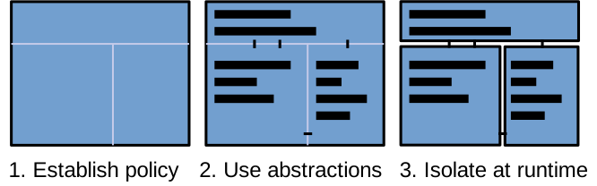
These steps are, in order:
- Establish a compartmentalisation policy: decide what part of the target software goes into what compartment.
- Use compartmentalisation abstractions to indicate in the code compartment boundaries, private/shared data and resources, to establish communication between compartments, and to secure interfaces. In the context of compartmentalisation, abstractions represent simplification layers that expose primitives for the programmer to express compartmentalisation policies within a program.
- At runtime, have an isolation mechanism enforce the partitioning between compartments.
We will cover the different ways to approach each step in detail in the next lectures.
Enforcing Isolation
The isolation between compartments is enforced at runtime with an isolation mechanism. A commonly used mechanism is the use of page tables, meaning that each compartment of a given application is placed within its own process. There are other mechanisms, implemented either in hardware or in software, that we will discuss in more detail in a subsequent lecture. Mechanisms restrict access to memory and system resources for each compartment to what is defined in the policy.
For example, focusing on memory accesses, in a compartmentalised application with two compartments, Comp1 and Comp2, using a hardware memory isolation mechanism (such as page tables), when Comp1 executes we could have the following:
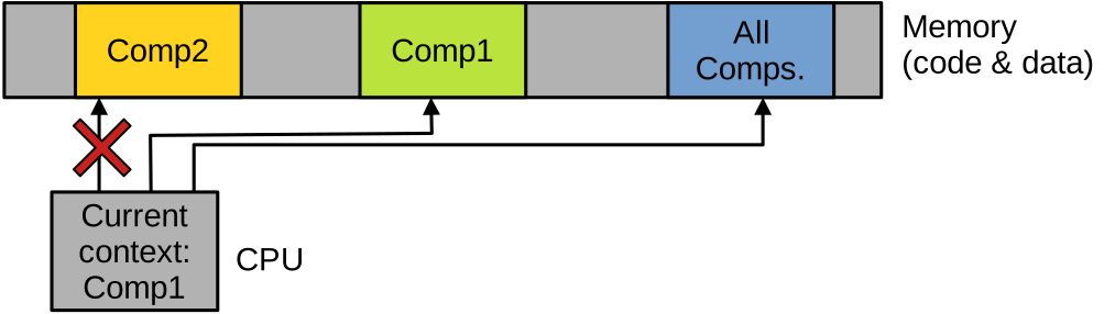
The memory allocated to the application is divided into three areas: one with code and data private to Comp1, another to Comp2, and an area of shared memory for communications between both compartments. When Comp1 runs, it can access its own private data and code, as well as the shared memory, but it cannot access Comp2’s private memory. When Comp2 runs, the permissions should be set up as follows:
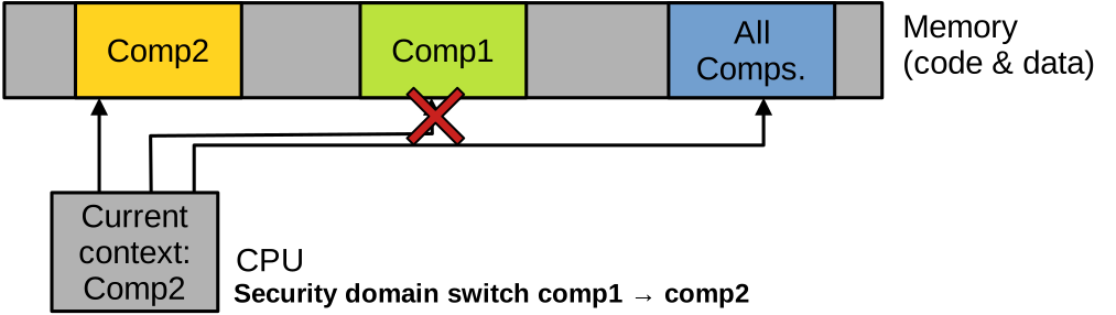
Most compartmentalisation approaches also need a privileged monitor. This is a secure piece of software that has ambient authority (i.e., it is part of the trusted computing base), and is used for various privileged operations, in particular to perform security transitions upon a compartment switch (for example, switching stacks and page tables).
The OS kernel can play that role, or, with certain mechanisms, it can also be achieved through a special privileged compartment. Because of its privileged nature, the monitor needs to be isolated from the other untrusted compartments.
Modern Compartmentalisation Approaches
Software compartmentalisation has been a known practice since at least the early 2000s and the publication of two seminal papers, Privman and Privtrans. Since then, it has not gained significant traction in the industry, for various reasons (e.g., engineering effort or performance impact) that we will detail in the next few lectures.
Recently, the appearance of new hardware isolation mechanisms has triggered renewed interest in compartmentalisation in the scientific community. Governments have been funding important research projects with up to tens of millions of GBP/USD to explore compartmentalisation, such as UKRI Digital Security by Design programme, or the US’ DARPA Compartmentalization and Privilege Management effort.
Examples of Compartmentalisation
To illustrate how an application can be concretely compartmentalised, consider the following code:
int global;

int library_function(int *parameter) {
  char *cryptokey = "private";

  int ret = *parameter + global + 42;
  return ret;
}

int main() {
  int arg = 100;
  global = 50;
  char *password = "secret";

  /* ... */

  int res = library_function(&arg);

  /* ... */

  return 0;
}
This is a monolithic application that is made of two functions, main and library_function.
Both functions operate on variables.
Some variables seem to be security-sensitive, e.g., cryptokey and password.
Other variables are accessed in both functions, e.g., global, as well as arg, whose address is passed from main to library_function.
We can compile and run it as follows:
$ gcc example-monolithic.c -o example-monolithic
$ ./example-monolithic
res: 192
Assume we would like to compartmentalise this application by applying a simple policy: putting library_function in one compartment, and main in the other.
This would ensure that if the code of one of the functions contains a bug exploitable by an attacker, the security-sensitive data (cryptokey for library_function, password for main) handled by the other function stays inaccessible to the attacker.
In terms of abstractions, we will use process-based isolation, placing each function of that application within its own process. That means we will use the page table mechanism to isolate the two compartments. The two functions communicate by accessing the global variable as well as exchanging a parameter and a return value, hence we will need to establish communication between the two compartments using IPC. We will explore two versions of the compartmentalised application, varying the communication mechanism: the first version will use pipes, and the second shared memory.
We will also present how the monolithic application could be compartmentalised using a hypothetical compartmentalisation framework.
Manual Compartmentalisation v1
We need to redesign the application to split it into two processes (i.e., our two compartments):
- Main function compartment.
- Library function compartment.
We also need to rework the code to make sure that the data that should be private to each compartment (in particular password and cryptokey) cannot be accessed by the other compartment.
Finally, we need to establish IPC-based communication between the two compartments to emulate access to a global variable global as well as the function call, which requires passing the value of arg from main to library_function, and returning ret from library_function to main.
Let us consider a first compartmentalised version of that application, using pipes for cross-compartment communications.
It is composed of the following files:
- The code for the
maincompartment, inexample-comp-pipe-main.c. - The code for the
library_functioncompartment, inexample-comp-pipe-lib.c. - A header file that will be included in both
.cfiles,example-comp-pipe.h, indicating the names of the pipes to use for communications.
The full sources for the entire compartmentalised application are available in this archive.
This is the common header file example-comp-pipe.h:
#ifndef EXAMPLE_COMP_PIPE_H
#define EXAMPLE_COMP_PIPE_H

#define PARAM_PIPE_PATH     "/tmp/param.pipe"
#define RESULT_PIPE_PATH    "/tmp/result.pipe"

#endif /* EXAMPLE_COMP_PIPE_H */
In this header file, we simply declare two constant strings indicating what files will be used to represent the pipes needed for communications.
Because a pipe is unidirectional, we need two pipes: one to send the value of global and the argument from the main compartment (i.e., process) into the library_function compartment when library_function is called, the other to send the return value the other way around once the function has completed.
This is the main function compartment example-comp-pipe-main.c:
#include "example-comp-pipe.h"
/* ... */
int global;

int main() {
  int arg = 100, send_fd, recv_fd;
  global = 50;
  char *password = "secret";

  mkfifo(PARAM_PIPE_PATH, 0666);
  mkfifo(RESULT_PIPE_PATH, 0666);

  pid_t pid = fork();
  if (pid == 0) {
    char *args[] = {"./example-comp-pipe-lib", NULL};
    char *envp[] = {NULL};
    execve("./example-comp-pipe-lib", args, envp);
    return -1;
  }

  // open pipe fds
  send_fd = open(PARAM_PIPE_PATH, O_WRONLY);
  recv_fd = open(RESULT_PIPE_PATH, O_RDONLY);

  // send param then global
  write(send_fd, &arg, sizeof(int));
  write(send_fd, &global, sizeof(int));

  // read the result
  int result;
  read(recv_fd, &result, sizeof(int));

  printf("res: %d\n", result);

  // wait for the child to finish
  wait(NULL);

  close(send_fd);
  close(recv_fd);
  return 0;
}
The beginning of the file looks very much like the original monolithic program, apart from the inclusion of example-comp-pipe.h, which contains the paths to the files that will represent the pipes used for communication with the other compartment.
We assume that the binary resulting from the compilation of this file (example-comp-pipe-main) will be the first to be executed to start the compartmentalised application.
After declaring and initialising a few variables, we use mkfifo to create the two pipes.
Next we use fork to create a new process, followed by a call to execve in the child to run the binary that corresponds to the second compartment, example-comp-pipe-lib.
Then we have the communications corresponding to what was a function call in our original monolithic program: we send with write on the first pipe the value of the argument, and the global variable that needs to be accessed by the second compartment.
The second compartment will run the code of library_function and, when that is done, will send the return value on the second pipe: we retrieve from that pipe the return value with read, and display the result.
This is the code for the second compartment, implementing the library function in example-comp-pipe-lib.c:
#include "example-comp-pipe.h"
/* ... */

int global;

int library_function(int *parameter) {
  char *cryptokey = "private";
  int ret = *parameter + global + 42;
  return ret;
}

int main() {
  int arg;

  int recv_fd = open(PARAM_PIPE_PATH, O_RDONLY);
  int send_fd = open(RESULT_PIPE_PATH, O_WRONLY);

  read(recv_fd, &arg, sizeof(int));
  read(recv_fd, &global, sizeof(int));

  int result = library_function(&arg);
  write(send_fd, &result, sizeof(int));

  close(recv_fd);
  close(send_fd);
  return 0;
}
This code is now a full program running in its own process, so we need a main function.
We start by opening the files corresponding to the communication pipes that should have been created by the first compartment when it was invoked.
Recall that the first compartment is supposed to be executed first, and that it creates the pipes before forking the second compartment.
We read from the first pipe the values of arg and global that we need to properly run the code of library_function, then call that function.
Once it is done, we send the return value result to the first compartment on the second pipe.
We can compile and run this first compartmentalised version as follows:
$ gcc example-comp-pipe-main.c -o example-comp-pipe-main
$ gcc example-comp-pipe-lib.c -o example-comp-pipe-lib
./example-comp-pipe-main
res: 192
It behaves similarly to the monolithic version.
Security Benefit of Compartmentalisation.
Notice that the security-sensitive data is only declared within the relevant compartment (password in the first compartment, and cryptokey in the second).
In that context, even if we assume a powerful attacker able to take over an entire compartment, they will still be unable to access the security-sensitive data present in the second compartment, because it is located in a separate process.
Manual Compartmentalisation v2
This second compartmentalised version of our example program uses shared memory for cross-compartment communications. Its structure is similar to the first: we have:
- The code for the
maincompartment, inexample-comp-shm-main.c. - The code for the
library_functioncompartment, inexample-comp-shm-lib.c. - A header file that will be included in both
.cfiles,example-comp-shm.h, declaring a data structure and indicating the name identifying the shared memory area used for communication.
This is the code of the common header example-comp-shm.h:
#ifndef EXAMPLE_COMP_SHM_H
#define EXAMPLE_COMP_SHM_H

#define SHM_NAME "/example.shm"

typedef struct {
    int param;
    int global;
    int result;
} shm_data_t;

#endif /* EXAMPLE_COMP_SHM_H */
This header file declares a data structure that will be held in shared memory and used for communication between the two compartments.
It contains all data flowing between the main and library compartments: the global variable, the function parameter, and the return value.
We also have the name identifying the shared memory: the manual page for shm_open indicates the format for such names: they should be of the form:
A null-terminated string of up to NAME_MAX (i.e., 255) characters consisting of an initial slash, followed by one or more characters, none of which are slashes.
Below is the code for the main function compartment, example-comp-shm-main.c:
#include "example-comp-shm.h"
/* ... */
int global;

int main() {
    shm_data_t *shared;
    int arg = 100;
    global = 50;
    char *password = "secret";

    // Create shm
    int fd = shm_open(SHM_NAME, O_CREAT | O_RDWR, 0666);

    // Map shm
    shared = mmap(NULL, sizeof(shm_data_t), PROT_READ | PROT_WRITE,
        MAP_SHARED, fd, 0);

    shared->param = arg;
    shared->global = global;

    pid_t pid = fork();
    if (pid == 0) {
        char *args[] = {"./example-comp-shm-lib", NULL};
        char *envp[] = {NULL};
        execve("./example-comp-shm-lib", args, envp);
        return -1;
    }

    // wait for the child to finish
    wait(NULL);

    printf("res: %d\n", shared->result);

    munmap(shared, sizeof(shm_data_t));
    close(fd);
    return 0;
}
This code initialises the first compartment and prepares for communication by creating the segment of shared memory with shm_open, and mapping it in the address space with mmap.
The size of this area of shared memory is that of one instance of a shm_data_t object.
In practice the OS will likely round it up to a full 4KB memory page, which is the granularity at which mmap operates.
Once the area of shared memory is ready, the first compartment writes in that area the values of the global variable (global) and function call parameter (arg) it wishes to communicate to the second compartment.
The first compartment then forks and uses execve to start the binary corresponding to the second compartment, which will access the shared memory to read arg and global, run library_function, and write its return value into shared memory.
The first compartment uses wait to ensure the second compartment is done before reading that return value in shared memory and printing it on the console.
The code below is for the library function compartment example-comp-shm-lib.c:
#include "example-comp-shm.h"
/* ... */
int global;

int library_function(int *parameter) {
    char *cryptokey = "private";
    int ret = *parameter + global + 42;
    return ret;
}

int main() {
    shm_data_t *shared;

    int fd = shm_open(SHM_NAME, O_RDWR, 0666);
    shared = mmap(NULL, sizeof(shm_data_t), PROT_READ | PROT_WRITE,
        MAP_SHARED, fd, 0);
    global = shared->global;

    shared->result = library_function(&(shared->param));

    munmap(shared, sizeof(shm_data_t));
    close(fd);
    return 0;
}
We use shm_open to open the shared memory area that was previously created by the first compartment, and map it in the address space with mmap.
The values of global and param are read from that area of shared memory, then library_function can be called.
We can then write the return value into shared memory.
This version behaves similarly to the monolithic one:
$ gcc -g example-comp-shm-main.c -o example-comp-shm-main
$ gcc -g example-comp-shm-lib.c -o example-comp-shm-lib
$ ./example-comp-shm-main
res: 192
As one can see, (re)designing for compartmentalisation, even on a simple example, can require quite a bit of engineering effort. The real effort required to compartmentalise a real-world application is in fact even (much) higher, because our example is overly simple:
- Only a small amount of data is exchanged between the compartments.
- That data does not need to be repeatedly accessed and updated by both compartments, so not much synchronisation or message passing is needed.
- We did not consider securing the cross-compartment interface (more on that in the next lecture).
Framework-Assisted Compartmentalisation
Research efforts have proposed compartmentalisation frameworks to ease the engineering effort required to compartmentalise applications. As we will see shortly, these frameworks can partially automate some of the tasks involved in compartmentalising an application. For example, the FlexOS framework only requires the programmer to use compiler annotations to indicate 1) shared data and 2) cross-compartment gates. After that, the code and data partitioning can be realised automatically. Below is an example of how to use FlexOS’ annotations to compartmentalise the monolithic application we studied above:
int __shared global;

int library_function(int *parameter) {
  char *cryptokey = "private";

  int ret = *parameter + global + 42;
  return ret;
}

int main() {
  int __shared arg = 100;
  global = 50;
  char *password = "secret";

  /* ... */

 int res = __gate(library_function, &arg);

  /* ... */

  return 0;
}
We aim for a similar policy to before: placing main in a compartment, and library_function in another.
Using FlexOS’ annotations, the programmer indicates shared data with the __shared keyword, marking as such global and arg.
The programmer also indicates compartment boundaries by placing gates where cross-compartment transitions need to happen, using the __gate keyword.
Software Compartmentalisation and Interfaces
You can access the slides 🖼️ for this lecture.
Retrofitting Compartmentalisation
We have seen that compartmentalisation is present in production only in a handful of specific use cases, such as micro-kernels, web browsers/servers, etc. These all represent software that was designed from scratch with compartmentalisation in mind. Another approach at compartmentalising applications is rather to retrofit it into existing monolithic software: there is a huge amount of legacy systems software code that would benefit from compartmentalisation.
Retrofitting compartmentalisation manually requires expert knowledge and represents a large amount of engineering effort, hence an ideal goal would be to compartmentalise monolithic software automatically:
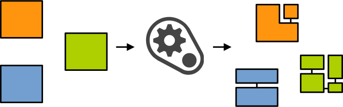
Automated Compartmentalisation
Automated compartmentalisation tools let the user compartmentalise seamlessly and without expert knowledge. Let us consider the different steps of compartmentalising an application, and reason about how easily these can be automated:
-
Policy Definition. Certain policy-definition approaches relying on standard programming language/runtime constructs can be at least partially automated, for example strategies placing every or particular libraries/object files/functions within their own compartments. Most policies that are manually defined aim primarily to isolate security-critical software components from low-trusted ones: some approaches can help automate that process, e.g., to identify trusted/untrusted code through static or dynamic analysis.
-
Abstractions: Identifying Cross-Compartment Shared Data. A particular challenge is to identify all shared data, i.e., data that needs to be accessed from several compartments. This is difficult but recent research efforts have proposed static analysis approaches that can provide an (over)estimate for the subset of data that needs to be shared in a compartmentalised application. Another abstraction-related task is the identification of cross-compartment boundaries in the code (e.g., by inserting gates), which is something that can be easily automated with static analysis once a policy is defined.
-
Applying an isolation mechanism: there are existing primitives (e.g.
fork()for processes) to automate isolation, and similar support for other mechanisms in several existing compartmentalisation frameworks. Establishing cross-compartment communications is also automatable once a mechanism has been selected and shared data has been identified: depending on the desired communication method, the automation technique will allocate such data in shared memory, or establish message-passing based communication channels between compartments.
Overall, although automation may not do as good a job as manual compartmentalisation, all the steps described above can be automated. However, there is a particular step of the compartmentalisation process that is still very hard to automate today: securing cross-compartment interfaces.
Interface Safety
Motivational Example
Consider the following monolithic program, that we would like to compartmentalise:
double data[DATA_SIZE];

  /* ... */

int lib_function(int index, double object) {
  data[index] = object;

  /* ... */
}

int main() {
  int index = get_index();
  double object = get_index();

  if (index < DATA_SIZE && index > 0)
    lib_function(index, object);

  /* ... */
}
In that monolithic version we do not trust the input source where index comes from, for example get_index may be getting it from the standard input.
Hence, there is a sanity check on the value of index before sending it as parameter to lib_function to avoid over/underflowing data.
Now assume that we want to compartmentalise that application according to the following policy: placing: lib_function in a compartment, main in another.
More precisely, we want to safebox lib_function, that we trust, from main that we do not fully trust.
Assuming we choose to compartmentalised using process-based isolation, we can simply partition the process into two processes, one running main and invoking the other running lib_function while passing it the necessary parameters index and object through some form of IPC.
The new (safebox) trust model we want to enforce leads to the emergence of a new internal trust boundary inside the application, that is the interface between the two compartments.
The existing sanity checks, that were written by the monolithic application developer that assumed that the entirety of the application’s code was fully trusted, are no longer sufficient.
If, as assumed by our trust model, the main compartment is malicious, we need to assume that the attacker can run arbitrary code in the context of that compartment, and execute instructions that are completely different from what is in the source code.
That can be achieved through code injection, control flow hijacking, return oriented programming, etc.
If main is compromised and sends corrupted values for the parameters passed to lib_function, this can lead to memory corruption in the context of the safebox, because there is no sanity checks enforced by the safebox on its input parameters, in particular on index.
In fact, an attacker taking over main gains an arbitrary memory write primitive within the safebox, which is a powerful attack tool.
A proper compartmentalised version of that application would introduce sanity checks on the trusted side, i.e., within the safebox, on the data flowing inside that compartment:
The lib_function compartment would look as follows:
double data[DATA_SIZE];

  /* ... */

int lib_function(int index, double object) {
  if (index >= DATA_SIZE || index < 0)
    return -1;

  data[index] = object;

  /* ... */
}
Interface Safety
The issue we illustrated in our example relates to interface safety. Enforcing interface safety corresponds to the integration, in compartmentalised applications, of sanity and validity checks on the data and control flow that exists between communicating distrustful compartments. As illustrated in our example, the lack of interface safety can provide ways for attackers to escape the compartmentalisation. In reality, we are going to see next that interface safety is in fact an absolute necessity, and that its absence negates most of the security benefits one would expect from compartmentalisation.
Our example also showed that retrofitting compartmentalisation creates internal trust boundaries, within monolithic software that was never designed with these internal trust assumptions:
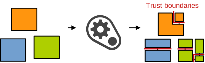
As a result, the number of issues related to interface safety is likely to be high. How bad is the problem? This is particularly concerning when the majority of existing approaches at compartmentalisation (including automated ones) do not provide any help for securing interfaces. With the aforementioned (ideal) goal of automating compartmentalisation, can we also automate the enforcement of interface safety?
Compartment Interface Vulnerabilities (CIVs)
CIV: Definition
The vulnerabilities that emerge due to the lack or absence of interface safety in a compartmentalised application, such as the one we saw in our example, are called Compartment Interface Vulnerabilities (CIVs). Through invalid and improperly-checked interface requests, a malicious compartment m can confuse a victim compartment v into misbehaving, and compromise some of the integrity, confidentiality, and availability guarantees expected from compartmentalisation. The main classes of CIV include:
- Data leakage: m can trick v into exposing some of v’s confidential data (e.g., cryptokeys, passwords, etc.) or addresses/pointer values.
- Data corruption: m can confuse v into dereferencing corrupted pointers (
NULLpointers, references to invalid data structures or unaccessible memory), using corrupted indexing information (with array indexing or pointer arithmetics), or using corrupted data structures. - Temporal violations: m can call functions exposed by v in the wrong order, and if both compartments run concurrently m can pass to v corrupted synchronisation primitives (e.g., locks) and perform TOCTTOU attacks in shared memory.
These issues can be triggered when m and v interact. m can either invoke v with invalid interface requests, e.g., invalid function call arguments or improper API usage ordering, but issues also emerge when v invokes m, which can feed v with corrupted return values or data referenced through pointer arguments. Issues regarding corrupted synchronisation primitives and TOCTTOU arise when m and v run concurrently. All types of attack are illustrated below:
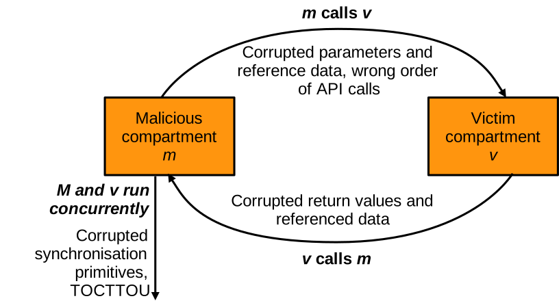
How Bad is the Issue of CIVs?
A recent research work proposes a tool named Conffuzz, which injects malformed data in monolithic software at potential compartment boundaries. The idea is to emulate the result of compartmentalising without securing interfaces, in order to study the impact of CIVs when interface safety is not properly addressed:
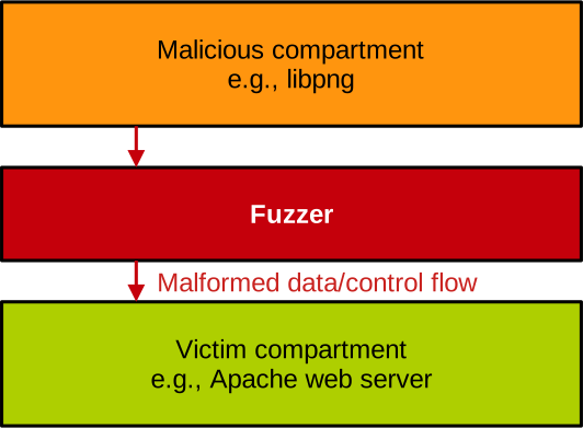
The fuzzer hooks into the program at a particular cross-compartment interface, e.g., between a main program and a library it links against. By corrupting the data flowing through that interface, the fuzzer emulates possible cross-compartment attacks by triggering a subset of the CIV types described above (mostly data corruption):
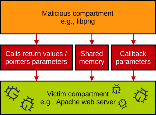
Conffuzz has been used to fuzz 36 APIs in total, divided into two trust models:
- Sandbox: Apache + libmarkdown (e.g., Apache is the trusted victim compartment, and libmarkdown is the untrusted malicious compartment), cURL + libnghttp2, git + libcurl, etc.
- Safebox: cURL + libssl (e.g., libssl is the trusted victim compartment and cURL is the untrusted malicious compartment), GPG + libgcrypt, sudo + libapparmor, etc.
The study mostly targets compartmentalisation policies at the library granularity, but also considers modules and internal APIs.
Many of these applications and libraries/modules/internal interfaces have been compartmentalised in past research studies.
The study uncovered a total of 629 unique CIVs, allowing the malicious compartment to perform limited or arbitrary memory accesses, in read, write or execute mode, in the context of the victim. It also uncovered additional CIVs consisting of allocation and NULL pointer dereference bugs.
Real-World CIV Example 1.
Here is an example of CIV, in the sudo application, with a compartmentalisation scenario in which the authentication API (victim compartment) is safeboxed from the rest of the program (malicious compartment):
int sudo_passwd_verify(struct passwd *pw, char *pass, sudo_auth *auth,
    struct sudo_conv_callback *cb) {
  /* ... abbreviated ... */
  sav = pass[8]; // read CIV
  pass[8] = '\0'; // write CIV
} /* ... abbreviated ... */
This code belongs to the sandboxed authentication API compartment, and that function can be invoked by the untrusted compartment containing the rest of the code.
If the size of the string pass passed by the untrusted main compartment is smaller than 8 bytes, the victim will read and write past the end of that buffer.
An interesting point to note is that, outside of compartmentalised scenarios, this bug can also be triggered by passing a password whose size is smaller than 8 bytes as input to sudo: this is CVE-2022-43995.
Real-World CIV Example 2. Below are two other examples of CIV, this time when the libssl cryptographic library is safeboxed:
// CIV 1: option setting API leads to arbitrary R/W
ulong SSL_CTX_set_options(SSL_CTX *ctx, ulong op) {
  return ctx->options |= op;
}
// CIV 2: cross-API object SSL_CTX with function
// pointers leads to arbitrary execution
SSL *SSL_new(SSL_CTX *ctx) {
  /* ... */
  s->method = ctx->method;
  /* ... */
  if (!s->method->ssl_new(s)) // arbitrary execution
    goto err;
} /* ... */
In the first CIV, the data referenced by ctx as well as the value of op are under the control of the malicious compartment, which gives the attacker a memory read and write primitive at arbitrary locations in the context of the victim (libssl) compartment.
In the second CIV, the malicious compartment controls the function pointer ctx->method->ssl_new(), dereferenced by the victim compartment, giving the attacker a powerful arbitrary code execution primitive.
Takeaways from the Study. The main conclusion from the study is that when compartmentalising without considering interface safety, CIVs are pervasive. In other words, compartmentalisation without securing interfaces is mostly meaningless.
Another insight from the study is that there are clear CIV disparities among different APIs. There is no correlation between API size and CIV count: there are large and almost totally CIV-free APIs, and small but fully vulnerable APIs. Further, some API design patterns (e.g. modules) are highly vulnerable because of a large amount of state exposure. In terms of impact, the study concludes that CIVs are high-impact: 75% of scenarios have at least 1 write vulnerability, and 70% of read/write CIVs and 50% of execute CIVs are arbitrary in nature, meaning they give an attacker memory access anywhere in the context of the victim compartment. Finally, the authors of the study note that fixing CIVs often goes beyond writing simple checks: it requires API redesign in many cases, something that is application-specific and hard to automate.
More details on the fuzzer, applications targeted, CIVs uncovered, and analysis are given in the paper.
Software Compartmentalisation Policies
You can access the slides 🖼️ for this lecture.
We have seen in the introduction that compartmentalising an application broadly involves three main steps:
- Determining a compartmentalisation policy.
- Implementing the compartmentalisation in the target application using abstractions.
- Enforcing at runtime the isolation between compartments using one or several mechanisms.
In this lecture, we cover policies.
Compartmentalisation Policies
What is a compartmentalisation policy? It is a series of choices made at the design stage when compartmentalising. More precisely, it is the definition, for a target application to compartmentalise, of how many compartments there should be, and what bits of the application go into what compartment. Assume we have an existing monolithic application to compartmentalise. As illustrated below, there are different possible compartmentalisation policies, and of course choosing a particular policy will have important consequences on the security and performance of the future compartmentalised application:
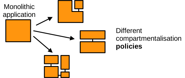
Compartment Selection Method
A first important choice regarding the policy is how to organise compartments. There are mainly two choices here:
- Code-centric or spatial approaches split the source code into different compartments. An example of a code-centric policy would be: put each library of the program within its own compartment. Another example is illustrated in the diagram below: we have a web server to compartmentalise, and choosing to put the main server code in one compartment and the SSL library in another is a code-centric compartmentalisation policy.
- Data-centric, also called temporal or horizontal, approaches rather place execution flows within their own compartments: for example, each thread or each process of an application is placed within its own compartment. You have an example below with our web server: imagine it spawns a certain number of worker threads, for example to handle requests concurrently. These workers execute more or less the same code, each running within its own compartment.
- Both methods can be combined into hybrid approaches. In our example below, we can place the main application’s code in one compartment, one library in a second compartment, plus additional compartments, one per worker thread.
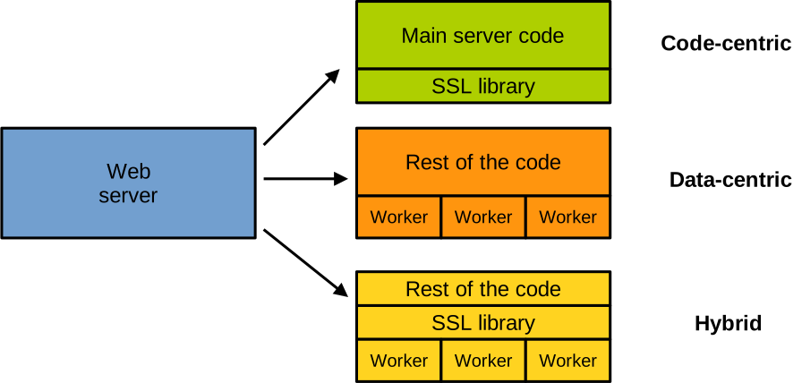
Compartment Granularity
The granularity of a compartmentalisation policy denotes how large or small compartments can be:
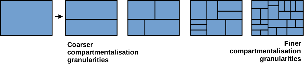
| Coarser granularities | Finer granularities | |
|---|---|---|
| Pros | Reduce compartmentalisation effort, lower performance impact | Better privilege reduction |
| Cons | Low degree of privilege reduction | Higher compartmentalisation complexity and performance impact |
From coarser to finer-grain we can compartmentalise at the level of library/software packages/subsystem, linkage units, functions, or even pieces of code within functions. Coarse granularity means that each compartment contains a large amount of code: generally this translates into a lower number of compartments, which reduces the compartmentalisation effort and the performance slowdown because there are less security domain switches. The degree of privilege reduction is also limited due to the large size of compartments. Fine granularity means having small compartments, which may translate into a large number of compartments. This is beneficial from the privilege reduction point of view, as it limits what an attacker can access when they subvert a single compartment. On the downside, a large number of compartments requires a lot of engineering to be put in place, and the many security domain crossings it involves at runtime can slow things down significantly.
Automating Policy Generation
As previously discussed, automation is an ideal goal in compartmentalisation. It would be ideal if we could take a monolithic program and give it to a framework, maybe a compiler, that would produce a compartmentalised version fully automatically, without any engineering effort or expert knowledge. In practice, existing production-ready or research approaches at compartmentalisation policy generation present various degrees of automation.
Manual Compartmentalisation. Most compartmentalised applications running currently in production have been partitioned fully manually.This requires an important amount of engineering effort, and entirely relies on the expertise of the programmers. Such approaches are also prone to human error, and it is difficult to prove that the resulting compartmentalisations are entirely correct. Still, one benefit of manual compartmentalisation is that an expert developer can precisely identify the components of an application that have low degrees of trust, and the components that are security sensitive. This leads to high-quality compartmentalisation policies, at the cost of a high engineering effort and correctness concerns.
Guided Manual Compartmentalisation. Such approaches assist developers with tools and feedback loops to reduce errors and improve boundary definition, while most of the policy definition effort stays manual. Typical aspects of the compartmentalisation that can be guided are the identification of security-sensitive or low-trust pieces of code and data.
Policy-refinement methods. With refinement approaches, the developer indicates high-level policies (e.g., “library A and library B should be within the same sandbox”), for example in a configuration file, or by marking untrusted and security-critical data with code annotations and letting the system make sure both categories do not end up in the same compartment. The frameworks supporting this method apply a good deal of automation; however, certain aspects of the job, such as securing interfaces, are still very hard to automate today and may require reworking of automatically generated policies.
- Full automation
- Requires no effort from the programmer.
- Computing data dependencies without manual refinement may lead to a weakened degree of privilege reduction.
- But full automation also raises concerns about lowered security guarantees.
- For example, it requires the extensive use of static analysis techniques which tend to overestimate: if such techniques are used to identify data that should be shared between several compartments, this will likely lead to a certain amount of oversharing.
Overall, the more automation is used, the lower the engineering effort is, but also the lower the security guarantees obtained from compartmentalisation will be.
Policy Languages
The ways in which policies can be expressed within the code of the compartmentalised program vary. Many existing compartmentalisation frameworks make use of code annotations, for example compiler attributes. These annotations allow things like marking some data as security sensitive or untrusted, marking data as private to a compartment or shared between multiple compartments, or indicating compartment boundaries. You have an example of annotations on the top right here, with a global reference marked as shared with a compartment, and a password variable marked as private to the containing compartment:
int function(char *parameter) {
  // treat all data as private by default,
  // mark shared data as such
  int __shared(compartment1) *glob_ref = // ...
  // or treat all data as shared by default,
  // mark private data as such
  char __private password[128];
}
Another approach is to use higher-level placement rules, for example the configuration file on the bottom right here places each library within its own compartment, and the rest of the code within an additional compartment:
# libredis, libopenjpg, and libxml each in a
# separate compartment, rest of the code in
# another compartment

default: comp0

libraries:
- libredis: comp1
- libopenjpg: comp2
- libxml: comp3
Overall, compartmentalisation frameworks let you express policy information in the code at various granularities, e.g., variables vs. entire libraries in our examples, and this also makes it more or less easy to enforce certain trust models over others. For example if we can only mark data as untrusted for sandboxing, but cannot mark data as security-sensitive, it’s unlikely that the framework in question supports the safebox isolation model.
Analysis Techniques
For approaches using automation, some analysis techniques must be used to determine permissions, compartment boundaries, and the status of data such as shared or private.
Static analysis is generally the default choice. It scales well to many applications and different policies, and, unlike dynamic analysis, it is complete, which is important. Unfortunately, it overestimates, which leads to issues such as oversharing when used to identify shared data. It can also be quite slow and resource demanding, and may not scale to very large code bases.
Dynamic analysis is, on the other hand, incomplete and underestimates: compartments may be underprivileged. This leads to permission faults at runtime under legitimate behaviour, which is not desirable in production. Overall, dynamic analysis offers good scalability to large programs (they just need to be executed), but poor scalability to many programs/policies (each combination needs to be executed).
A few hybrid methods have been presented, but overall static and dynamic analysis do not compose well. Indeed, when you mix them, you obtain a mix of the drawbacks of both approaches, which is not ideal.
Programming Language Genericity
The vast majority of policy definition methods are not generic and focus on one or a class of programming languages. This is because they need to tackle specific problems, such as pointer aliasing in C, but also because many approaches leverage language-specific features. For example the RLBox framework focuses on C++ and uses the rich type information exposed by the language to partially automate some interface safety checks, something not available in other languages, e.g., C. Another example is the software fault isolation model applied to WebAssembly sandboxes, which is limited to the many languages supported by this runtime.
Software Compartmentalisation Abstractions
You can access the slides 🖼️ for this lecture.
Here we cover the abstractions used by programmers to implement compartmentalisation policies in applications.
Abstractions
Abstraction is a term commonly used in computer science. An abstraction refers to a simplification layer whose goal is to ease the use of a software or hardware component. The abstraction will hide all the unnecessary internal details of the component in question, and will expose a convenient and clear interface for it to be invoked.
Let us illustrate the concept with an example. We have a complex component that has a lot of different functionalities. We can create an abstraction that somehow handles all of these different functionalities, and exposes them under a higher-level, simpler interface for clients to use:
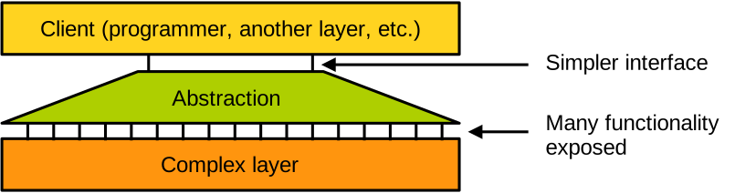
Here the client can be the programmer, another software or hardware layer, etc. Another concrete example is that of an operating system, e.g., the Linux kernel. The kernel itself implements tons of functionalities, remember that it is made of more than 20 million lines of code. The system call interface abstracts all these functionalities for user space applications under a relatively small interface made of a series of system calls that can be invoked to request any service from the OS. In other words, the system call interface is an abstraction of the operating system (complex layer) for client applications (client).
Abstractions are absolutely everywhere in computer science. We can list a few more examples of abstractions:
- A programming language is an abstraction of assembly instructions, simplifying the development of programs using high-level statements, functions, loops, etc.
- Each system call is an abstraction of relatively complex features implemented by the operating system; for example, the
forkUNIX primitive, implemented through the Linuxclonesystem call, abstracts many details of process creation and resource duplication. - A file is an abstraction of data stored on disk, indexed with a particular path on the filesystem. The operations one can apply to a file, such as reading from or writing to it, abstract away complex mechanisms such as drivers communicating with devices following specific protocols, block allocation, request scheduling, data and metadata caching, etc.
Compartmentalisation Abstractions
A compartmentalisation abstraction is a simplification layer that exposes primitives for the programmer to express compartmentalisation policies within a program. Using such abstractions, the programmer can express many things:
- What part of the application goes into what compartment.
- What and where are the compartment boundaries.
- What data should be shared between compartments, or private to the containing compartment.
- When and how compartments should be created and destroyed.
- How to manage compartments’ permissions.
- Etc.
Main Abstraction Categories
The compartmentalisation abstractions one can use are very different depending on what compartmentalisation approach, framework and tools one decides to use. However, most abstractions will fall within one of the following main categories:
CREATEandDESTROYfor compartment creation and destruction.ASSIGNto assign permissions to a compartment.CALLandRETURNto invoke the execution of and return from a compartment.
CREATE, DESTROY, ASSIGN Abstractions
The first category is CREATE and DESTROY: the programmer needs a way to express the creation and destruction of compartments in the code.
They are illustrated in steps 1 and 2 in the diagram below:
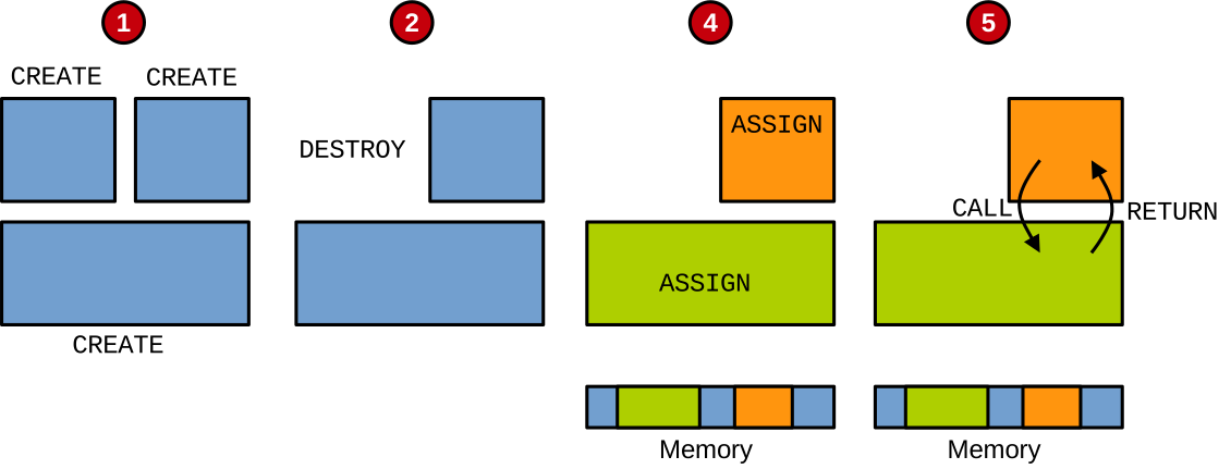
Examples of abstractions belonging to the CREATE and DESTROY categories are calls to fork and exit, if one chooses to use process-based compartmentalisation.
Another important category of abstraction is ASSIGN.
It corresponds to abstractions that let the programmer assign permissions to compartments.
For example, as illustrated in step 3 in the diagram above, we could have a part of the memory be accessible only by the green compartment, and another part of the memory accessible only by the orange one.
We’ll see in the next lecture that there are several mechanisms that allow us to enforce these permissions.
An example would simply be again to run each compartment within its own process; this way they would have separate address spaces.
CALL/RETURN Abstractions
Because they belong to the same application, at some point compartments need to communicate with each other and transition execution from one to another.
These cross-compartment transitions are security domain switches, realised with abstractions belonging to the CALL and RETURN categories, as illustrated in step 4 in the diagram above.
If we zoom in on CALL and RETURN abstractions, they will generally enforce a series of security properties.
First, we need some form of control flow integrity between compartments: we cannot let an untrusted caller compartment jump to arbitrary code addresses within another callee compartment; that would be equivalent to letting the caller execute arbitrary code within the context of the callee.
Hence, CALL and RETURN abstractions must make sure that cross-compartment transitions only target legitimate locations in the code.
For example, a compartment should only be called through the API it exposes.
Another important aspect of CALL and RETURN abstractions is that they must switch the CPU state from that of the caller compartment to that of the callee’s, e.g., switch stacks and clear registers, as part of the cross-compartment transitions.
Without this, the old stack and register content may contain important information that would leak across compartments.
CALL and RETURN abstractions can be synchronous or asynchronous.
With synchronous calls and returns, compartment switches are relatively similar to function calls and returns: the caller compartment blocks waiting for the callee to return.
This is illustrated on the left of the diagram below.
If the compartments run concurrently, CALLs and RETURNs can also be asynchronous, meaning that the caller does not wait for the callee to finish processing the call.
This is illustrated on the right of the diagram.
In that case, the application is closer to a distributed system, and transitions between compartments become remote procedure calls involving message-passing communication.
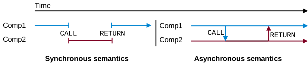
Implicit/Explicit Abstractions
Abstractions can be explicit, meaning they are exposed to the programmer, who must explicitly use them, for example by placing annotations. This involves a certain amount of engineering effort, depending on how easy it is to use the abstractions. Abstractions can also be implicit, requiring no intervention from the programmer because they are applied automatically. For example, you could have a compartmentalisation framework placing each library within its own compartment and automatically handling compartment creation, destruction, and transitions.
Because most existing approaches to compartmentalisation are code-centric, CREATE and DESTROY abstractions are often implicit and managed automatically.
For example, when placing a library within its own compartment, that compartment will be created when the application starts, and destroyed when the application exits.
The more automated an approach is, the more implicit abstractions it will support, including ASSIGN, CALL and RETURN.
Properties Enforced
Most of the existing software compartmentalisation abstractions will at least enforce integrity, which is a prerequisite to enforce the other properties (confidentiality, availability). Confidentiality is also a property commonly enforced.
Concerning availability, it is not supported by most abstractions.
The reason why there is almost no compartmentalisation work targeting availability is rather simple: it is extremely difficult to achieve, and in most cases it requires entirely redesigning the application one wishes to compartmentalise from scratch.
Indeed, to be able to preserve availability in the presence of one or more malicious components, the application needs to be reworked into a fault-tolerant distributed system.
That requires specific abstractions: compartments need to run concurrently, and CALL/RETURN abstractions need to be asynchronous.
We need to enforce performance isolation and bounded resource consumption across compartments, because we can’t let a malicious compartment starve the rest of the application of resources.
The TCB as well as the interfaces need to be redesigned to place as much state as possible outside of compartments that may be prone to crashes, because we want to be able to restart them in the case they fail.
All of this is obviously extremely complicated, and that complexity needs to be added on top of the difficulty of maintaining confidentiality and integrity, which is already quite hard.
Composing with Other Abstractions
One last important consideration about compartmentalisation abstractions is how they compose with other system abstractions.
Processes and Threads
For example, regarding threads and processes, they can either be orthogonal to compartments, with one thread or one process able to execute multiple compartments, and compartment transitions realised in the context of the thread or process. This is illustrated on the left of the diagram below, with two threads running several compartments, transitioning upon calls and returns:
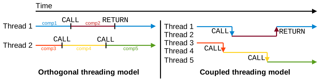
Processes or threads can also be coupled with the compartments.
In that case, each process or thread executes a single compartment only, and upon CALLs and RETURNs the running thread or process needs to be switched.
This is illustrated on the right of the diagram above.
CPU privilege levels
When compartmentalising an application, the abstractions used are influenced by the user/kernel interface. In particular, as many compartmentalised systems require a privileged monitor to perform security domain transitions, the kernel can play that role. This is the case implicitly when using process-based compartmentalisation. The monitor can also be placed in user space, which may have some performance benefits or drawbacks, depending on how the monitor is implemented and isolated.
When compartmentalising the kernel or another privileged entity like a virtual machine monitor, things are more complicated because these entities run with full privileges, but we need to reduce some of these privileges for certain compartments. The goal here is to establish a trusted computing base that will play the role of the aforementioned monitor, and to isolate it from the rest of the kernel or the hypervisor.
Monitor-Level Side Channels
The isolation mechanisms used for compartmentalisation, which we will cover in the next lecture, are quite robust, and in most cases, combined with good interface security, they will prevent compartment A from directly accessing the private memory of compartment B. Yet another attack vector is the secure monitor, which in many cases is the kernel. If not properly secured for compartmentalisation, some kernel interfaces may allow a malicious compartment to access memory supposed to be private to other compartments:
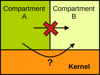
Kernel interfaces are well secured when considering process-based compartmentalisation, because the kernel is already designed to provide good isolation between processes.
But when using some of the more modern isolation mechanisms, these interfaces may become concerning, because the kernel was not designed with these isolation mechanisms in mind.
Examples of such monitor (kernel) level side channels, which may allow the isolation enforced by certain mechanisms to be bypassed, include the system call interface (e.g., a malicious compartment able to mmap memory from another victim compartment), or pseudo-filesystems (e.g., a malicious compartment having access to /dev/mem, which holds the contents of all physical memory).
Software Compartmentalisation: Isolation Mechanisms
You can access the slides 🖼️ for this lecture.
This last lecture on compartmentalisation covers the various mechanisms that can enforce the isolation between different compartments.
Compartmentalisation Mechanisms
A compartmentalisation mechanism enforces at runtime the isolation between compartments, as defined by policies and implemented through abstractions. All the mechanisms one wishes to use for compartmentalisation must allow the following two high-level properties: First, compartments represent different protection domains and the mechanism should provide proper isolation between them, i.e., prevent a compartment from reading, writing, or executing data and code in the memory of another compartment:
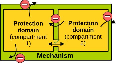
Second, the mechanism should allow safe and controlled communications between compartments that need to communicate.
In other words, the CALL and RETURN abstractions we previously mentioned should be implementable with the considered mechanism.
The mechanism should also ensure a form of cross-compartment control flow integrity: communication should allow compartment A to invoke compartment B only through well-defined interfaces, and not at arbitrary points in B’s code.
Ideally, the data exchanged between compartments should also be limited to the data required for communication: anything more than that would be oversharing, which decreases the level of security.
Examples of Mechanisms
Several mechanisms can be used to enforce the isolation required in a compartmentalised scenario. They can be classified into two categories: hardware and software mechanisms.
Hardware Isolation Mechanisms. We have already mentioned several times process-based compartmentalisation, where each compartment runs within its own process. In that case, the mechanism used to isolate compartments is the page tables. Another mechanism that isolates the kernel from user space uses the privilege levels on the CPU. Memory protection keys is another mechanism that allows creating multiple compartments within a single address space. We also mentioned previously trusted execution environments and confidential VMs, which provide strong isolation even in the presence of malicious privileged layers such as the OS. Other examples of hardware isolation mechanisms include bound-checking hardware or hardware memory capabilities.
Software Isolation Mechanism. Software Fault Isolation (SFI) is a compiler-level technique, in which the code of compartments is generated in such a way that it cannot escape a sandbox. Control transitions such as jumps or calls are also generated in such a way that they can only target legitimate code locations, enforcing control flow integrity. Memory safe languages can be seen as a form of isolation mechanism that prevents the memory safety issues we covered previously, which could allow a compartment to access memory it is not supposed to. Finally, bounds-checking software such as FAT pointers augments the pointers with information about the bounds of the objects they point to. When these pointers are dereferenced, these bounds are checked before the access occurs, which gives more guarantees that a compartment will not be able to access memory it is not supposed to read or write.
Hardware vs. Software Isolation. Most modern compartmentalisation approaches rely on hardware mechanisms. That is because such mechanisms can provide isolation that is both strong and relatively fast. Several hardware mechanisms are also compatible with many types of software, regardless of the language in which it is written. Conversely, software mechanisms are available everywhere, regardless of the hardware. However, they are generally slower and suffer from compatibility issues.
Cross-Compartment Communications
In a compartmentalised application, compartments are not entirely isolated and need to communicate.
With that in mind, isolation mechanisms must support some form of CALL and RETURN primitives to transition between compartments.
In addition to that, the mechanisms should also support a way to exchange data between compartments upon such transitions.
For example, to pass parameters or return values when there is a cross-compartment call, and also to handle the data pointed to by reference parameters exchanged across compartments (if any).
To achieve data exchange there are 2 main methods: message passing and shared memory.
Message Passing. The first class of cross-compartment data exchange methods is message passing: the data is sent and received between compartments over some form of communication channel, generally involving one or more data copies. This is the case with IPCs such as pipes or sockets, when using process-based compartmentalisation. Message passing is relatively slow because of the data copies it involves, and also sometimes because of the need to marshal/unmarshal transmitted/received data into/from a format suitable for communication. Message passing is also very secure, because a particular piece of data is never accessible from more than one compartment at a time (no possibility of Time of Check to Time of Use – TOCTOU – attacks).
Shared Memory. The second method for data exchange is shared memory. Compartments can establish a portion of shared memory, so they can share part or even their entire address space. Doing so, they don’t need to send and receive data; they simply need to send and receive references to that data, which are much smaller. Hence, shared memory has the potential to be much faster than message passing. However, it is also less secure. In scenarios where compartments run concurrently, because two communicating compartments can access the memory they share at the same time, there is a risk of race conditions and TOCTOU attacks.
Most mechanisms will allow one or both approaches. For example, as seen with our example program in the introduction to the topic of compartmentalisation, processes can either share memory or establish message-passing-based IPCs (e.g., pipes).
Trust Models
Each mechanism is designed with a specific trust model in mind. For example, CPU privilege levels target single-direction distrust: the kernel distrusts the application, which itself trusts the kernel. Other mechanisms target mutual distrust, such as the page table establishing different address spaces for different processes, or trusted execution environments. Mechanisms will also influence the content of the trusted computing base (TCB). In general, from the point of view of a compartment, the TCB will contain at least the compartment’s code, the system’s loader, the motherboard firmware, BIOS, the OS and hypervisor and their boot processes, as well as the machine’s physical environment. Some mechanisms, like trusted execution environments, allow reducing that TCB by removing the OS and hypervisor.
Mechanisms: Misc. Aspects
A few more aspects regarding mechanisms are worth discussing. Mechanisms will enforce different permissions, generally a combination of read/write/execute, but also address – in the sense of the ability for a compartment to create a reference to a resource or an area of memory. Not all mechanisms support all permissions: for example, Intel’s implementation of memory protection keys supports only enforcing read/write access, read-only access, or no read/write access at all, and there is no support for preventing execution.
The enforcement granularity varies depending on the mechanisms. Some, like the page tables, will allow or deny memory accesses at the granularity of 4KB memory pages. While others, such as bounds-checking software, will provide byte-level memory protection. These considerations have implications in terms of memory consumption and oversharing for compartmentalised applications using these mechanisms.
Certain mechanisms also support a limited number of domains, for example 16 only with Intel Memory Protection Keys. With MPK this number can be increased with some forms of virtualisation, at the cost of a non-negligible performance slowdown. Other mechanisms, such as processes, support an unbounded number of domains. More generally, the more compartments you have, the more scalability issues arise.
Performance Considerations
Choosing a particular mechanism for a compartmentalisation project has an important impact on the compartmentalised application’s performance. The mechanism impacts performance overheads as it defines the time taken for security domain switches, the cost to communicate data across compartment boundaries, and possibly the cost to sanitise such communication data. Creating and destroying compartments may have non-negligible performance costs, as does setting up and updating compartments’ permissions. The way memory needs to be organised to ensure the shared or private nature of data will impact performance due to memory fragmentation, access locality, and its impact on the caches. Finally, as mentioned previously, scalability issues may arise due to too many compartments, or compartments that are too large.
Today, the main source of performance concerns remains the domain switching latency. For that reason, the most up-to-date compartmentalisation approaches rely on mechanisms that work within a single address space to avoid context switches, and that can also perform security domain switches without relying on an exception, contrary to something like system calls.
Software Compartmentalisation: Further Readings
- Lefeuvre et al., SoK: Software Compartmentalisation. Modern and high-level overview of the field. Heavily inspired this week’s content. References 250+ compartmentalisation paper.
- Kilpatrick, Privman: A Library for Partitioning Applications. Seminal work on compartmentalisation.
- Provos et al., Preventing Privilege Escalation. Another seminal work.
- Watson et al., CHERI: A hybrid capability-system architecture for scalable software compartmentalization. An isolation mechanism tailored for efficient - compartmentalisation. More on CHERI in the hardware part of the unit.
- Lefeuvre et al., Assessing the Impact of Interface Vulnerabilities in Compartmentalized Software. Explores the problem of securing cross-compartment interfaces.
- Watson et al., Capsicum: practical capabilities for UNIX.
Introduction to Virtualisation
You can access the slides 🖼️ for this lecture.
Definition
Let’s start with a simple definition of virtualisation. It is not really complete, but it is a good starting point:
Virtualisation technologies are the set of software and hardware components that allow running multiple operating systems at the same time on the same physical machine
The type of virtualisation we’ll discuss in this unit mostly concerns the goal of running several operating systems (OSes) on the same physical machine. A fundamental challenge here is that by design an operating system expects to be the only privileged entity with total control over the hardware on a computer. In other words, an operating system is not designed to run alongside and share a machine with other operating systems. In that context, how can 2 or more OSes cohabit on a single machine?
To address that problem we use a combination of hardware and software to create a series of virtual machines (VMs) running on a given physical machine, and we run each operating system within its own VM. That way we give the illusion to each OS that it is running alone and in total control on its VM:
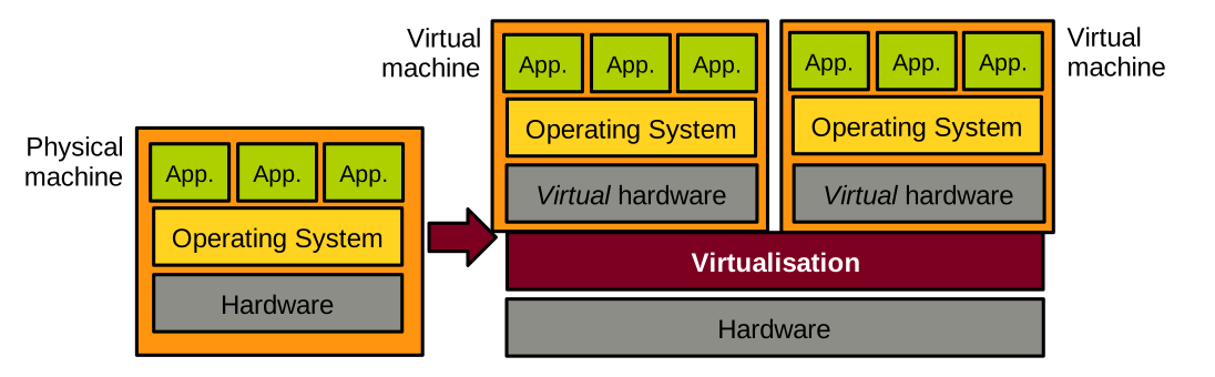
For this approach to work, the virtualisation layer needs to achieve three fundamental high-level objectives, illustrated below:
- The speed of an OS should be the same when running in a VM vs. running natively. The same applies to user-space applications running on top of that OS.
- The code of an existing OS supporting native execution should not have to be updated to run in a virtualised environment. The same applies to the applications.
- The OSes running virtualised on a physical machine should not be able to interfere with each other. For example, they should not be able to access each other’s memory. A virtualised OS should not be able to bottleneck resources such as CPU, memory, or I/O at the expense of the other virtualised OSes running alongside it.
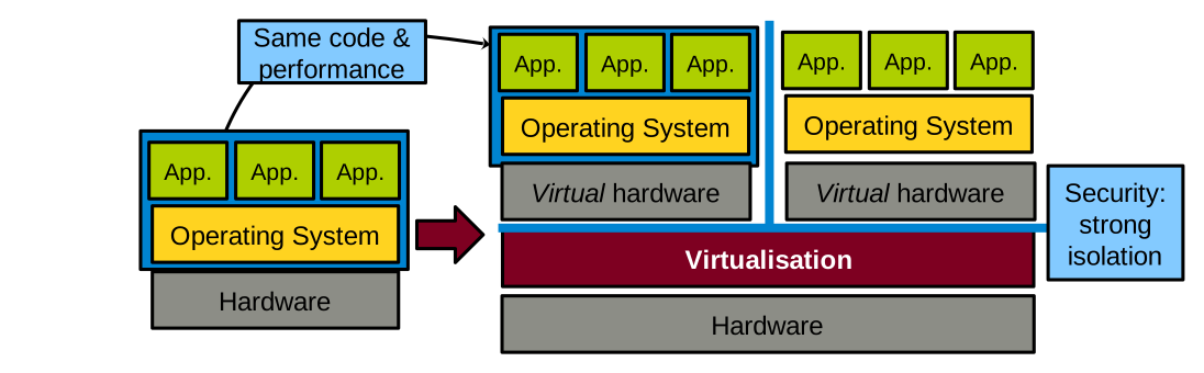
Points 1 and 2 above are necessary for adoption: businesses are unlikely to adopt virtualisation solutions if the performance hit is too high, or if it means changing OSes and applications, which is a significant engineering effort. Point 3 relates to security: virtualised OSes running on the same physical machine are often controlled by distrusting parties, and the virtualisation layer must enforce isolation guarantees.
A Bit of History
In the 1960s IBM produced System/360 (S/360), a family of computers of various sizes (i.e. processing power) built using the same architecture. A client could buy a small model for testing/prototyping, and a large mainframe later. Following that model, clients often realised they wanted to take a set of software applications running on multiple small models and run them all on a single large model. This is called consolidation, and it is one of the main use cases for virtualisation.
14 models were produced between 1965 and 1978. The model 67 introduced a virtualisable architecture: a physical machine of that model could appear as a set of multiple, less powerful versions of itself: virtual machines (VMs).
In 1974, a seminal paper on the topic of virtualisation was published: Formal Requirements for Virtualizable Third Generation Architectures.
This paper, co-authored by computer scientists Gerald J. Popek and Robert P. Goldberg, listed the requirements for an Instruction Set Architecture (ISA) to be virtualisable. It also described the properties that the systems software managing virtual machines (the virtual machine monitor or the hypervisor) must have for virtualisation to be possible on that ISA. We will study that paper in detail in one of the next lectures. Indeed, the principles defined in this paper are still relevant today, and they have guided the design of modern virtualisable ISAs such as Intel/AMD x86-64, ARM64, or RISC-V.
At the time the Popek and Goldberg paper was published, virtualisation was not in high demand. In the 1990s and early 2000s, that changed. A growing need for virtualisation was motivated by various factors: the rising need for workload consolidation, the continuous increase in computing power, or the boom of data centres during the dot-com bubble. The problem was that the most widespread ISA at the time, Intel x86-32, was not properly virtualisable based on the requirements described in the Popek and Goldberg paper. At that time, several software-based virtualisation solutions trying to virtualise x86-32 by overcoming the ISA’s limitations came out of academic research: Disco from Stanford, and Xen from Cambridge. These solutions later transitioned to the industry: the authors of Disco founded VMware, and Xen was for a long time the main virtual machine monitor used by Amazon Web Services.
In the 2000s, the demand for virtualisation exploded. The modern ISAs that we still use today were designed with virtualisation in mind, following the principles defined by Popek and Goldberg. These ISAs include hardware support for virtualisation, which is leveraged by today’s virtual machine monitors such as Linux’s KVM, VirtualBox, Microsoft’s Hyper-V, or the current versions of Xen.
Use Cases
Consolidation
Consolidation consists in taking a set of software applications, e.g. a web server, a mail server, and other software, initially running on X physical machines, and running everything on a smaller set of Y physical machines (Y < X) — possibly even a single machine, by creating X virtual machines.
As previously mentioned, this is the historical motivation for developing virtualisation technologies.
Consolidation gives most of the benefits of multi-computer systems without the associated financial and management costs. The financial savings are clear: we need to buy fewer computers. The management savings include saving space and reducing the workload for system administrators by having fewer machines.
The benefits of multi-computer systems that can be maintained on a single or small set of machine(s) include:
- Heterogeneity of software dependencies: if we have several applications with different dependency needs in terms of operating system/library models and versions, it is easy to run each application within its own virtual machine set up with the proper environment for that particular application. Environments from different virtual machines do not need to interfere with each other, and can evolve independently along with the needs in terms of dependency updates.
- Reliability: if one application crashes the system through a bug/resource hog, the fault will be contained within the VM and will not affect other virtual machines running on the same host.
- Security: same as for reliability, if one application gets hacked and the attacker manages to take over the operating system, the attack will still be confined to the containing VM and the attacker won’t be able to access other VMs running on the same host.
Software Development
Virtualisation offers significant advantages for software development by enabling multiple VMs to run on a single physical host, each with its own operating system and system libraries. This flexibility allows developers to emulate diverse environments without the need for multiple physical machines. For example, a developer working on a Windows machine but developing software for the Linux kernel features can use a VM to run different Linux distributions on the same host, ensuring compatibility and testing across versions.
Provisioning VMs is rapid and cost-efficient compared to setting up physical hardware, making it ideal for iterative development and continuous integration workflows. Furthermore, VMs are self-contained units that encapsulate the entire software stack including the operating system, libraries, and dependencies: they provide a reliable and reproducible environment for development, automated testing, and even deployment. This isolation reduces configuration conflicts and simplifies collaboration across teams.
These are the logos of a few technologies that are extensively used in software development:

- VirtualBox and VMware Workstation can run a Linux VM on a Windows host for Linux development without the need to install Linux natively.
- Vagrant allows automating the provisioning (installation) of one or several VMs for quick iterations of the development/testing/deployment cycle.
- Docker creates containers that are VM-like environments that can be set up automatically and almost instantaneously. We’ll talk more about containers later in this course unit.
Migration, Checkpoint/Restart
The state of a running VM is easily identifiable, hence it is relatively simple to checkpoint/restart and live-migrate that VM.
Checkpoint/restart consists in taking a snapshot of the VM’s state and storing it on disk. That snapshot can then be restored later for the VM to resume in the exact same state it was when the snapshot was taken. This is useful when executing long-running jobs (e.g. HPC applications, ML training, etc.): their progress can be saved with this technique to avoid restarting the entire job in case something goes wrong during their execution (e.g. crash).
Live migration consists in moving a VM from one physical host to another transparently, i.e. without the VM’s users noticing it: there should be no need for reconnecting, and no noticeable performance drop during the migration. This is useful in many scenarios, e.g., to free resources for maintenance, power saving, load balancing, or when a fault is expected.
Both checkpoint/restart and live-migration are straightforward to realise with a VM. This is in opposition to checkpointing/migrating an application/a process, which is more complicated because the state of an application is made of many elements (including a lot of kernel data structures) that are hard to properly identify.
This seminal paper on VM live migration is worth a read: Clark et al., Live Migration of Virtual Machines, NSDI’05.
Hardware Emulation
Emulation allows creating virtual machines whose CPU has an architecture (ISA) that is different from that of the host computer. This is useful for software development or to provide backward compatibility. A few examples are illustrated below. The development frameworks for smartphone applications (iOS/Android) are generally used on standard desktop/laptop machines running Intel x86-64 CPUs, and allow the creation of virtual machines representing smartphones, which generally embed ARM64 CPUs, for testing purposes. Modern video game consoles provide some degree of retro-compatibility with previous generations; for example, the Xbox Series X, released in 2020, can run Xbox 360 games that came out starting in 2005. Emulation can also let users create virtual machines for hardware that is not widely available anymore on modern hardware, e.g. old arcade machines.
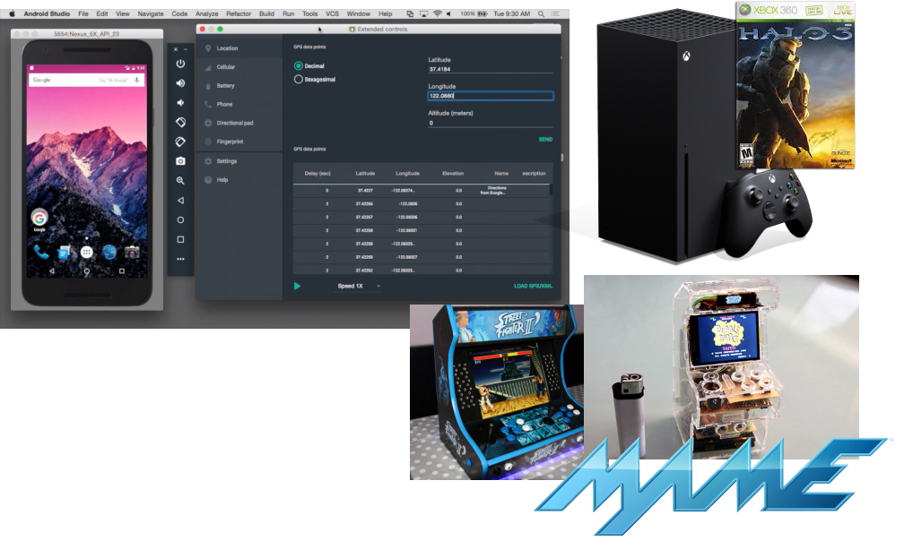
Cloud Computing
Virtualisation enables cloud computing, a computing paradigm in which cloud providers own a large quantity of computing resources (server farms) and provide remote access to these resources to their clients, known as tenants. This allows tenants to offload local computing workloads to the provider’s infrastructure. Tenants share access to the provider’s resources, and it is common for multiple clients of a cloud provider to execute their workload on the same physical host. Because, as a general rule, tenants do not trust each other, it is very important for the resource sharing enabled by the cloud to be secure: the entire cloud business model relies on the proper isolation between tenants’ workloads. Imagine if there was no such isolation between two distrusting clients whose workloads are co-located on the same host. One of these clients may be able to read and/or modify the code/data related to the other’s workload, which would negate most of the benefits of cloud computing.
This strong isolation required between tenants’ workloads is achieved by placing their applications in separate virtual machines. As we will see next, security/strong isolation between VMs is one of the design principles of virtualisation.
There are several ways for clients to leverage the cloud:
- Infrastructure as a Service (IaaS), in which clients rent VMs running on the provider’s infrastructure to run their workloads, e.g. a web server.
- Platform as a Service (PaaS), in which tenants develop and deploy their own applications using dedicated cloud frameworks, e.g., Google App Engine.
- Software as a Service (SaaS), where clients replace a commonly-used local service (e.g. an internal web server) with the cloud provider’s solution, e.g. using Gmail or Outlook 365 for emails.
- Function as a Service (FaaS), a newer paradigm in which developers deploy on the provider’s infrastructure individual functions that run on demand and automatically scale without managing servers.
The main goal of cloud computing for tenants is to save on management, infrastructure, development, and maintenance costs. Below are a few logos of popular services: AWS EC2 (IaaS), Google App Engine (PaaS), Gmail (SaaS) and AWS Lambda (FaaS):

Security
Because the isolation between the virtual machines running on the same host is so strong, virtualisation has many security applications beyond cloud computing.
Sandboxing confines an untrusted workload within a VM, ensuring that it cannot access the rest of the host’s resources. Beyond the obvious need for that in cloud computing, sandboxing is also useful when doing virus/malware analysis, running honeypots, and more generally running any piece of code that is not fully trusted (e.g., executables downloaded from the internet). Qubes OS, whose logo is illustrated below, is a security-focused desktop operating system that uses virtualisation to isolate each application into a separate VM to reduce the impact of security breaches.

VM introspection consists in analysing the guest’s behaviour from the host. This is quite useful in security-oriented scenarios; however, it can be a difficult task because of the lack of visibility into what is going on inside a VM when viewed from the host.
Virtualisation: In-depth Definition
Let’s now see a more in-depth definition of the concept of virtualisation. It is adapted from Hardware and Software Support for Virtualization by Tsafrir, Bugnion and Nieh:
Virtualisation is the abstraction at a widely-used interface of one or several components of a computer system, whereby the created virtual resource is identical to the virtualised component and cannot be bypassed by its clients
This applies to a virtual machine: the abstraction at the software (OS)/hardware interface. The virtual machine presents to the OS a set of virtual hardware which is identical to its physical counterpart, so existing OSes designed for physical machines can run as is in a VM. Guest OSes cannot escape this VM abstraction: as we will discuss, the isolation between a VM and the virtualisation layer or other VMs is very strong.
Multiplexing, Aggregation, Emulation
Virtualisation, in its general definition, is achieved by using/combining three main principles:
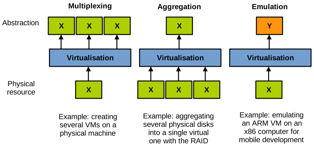
- Multiplexing consists in creating several virtual resources from a single physical resource. A well-known example of multiplexing is the creation of several VMs on a single physical host machine.
- Aggregation consists in pooling together several physical resources into a single one. An example here is RAID, which groups together several storage devices into a single one with higher performance/capacity/reliability.
- Emulation consists of creating a virtual resource of type Y on a physical resource of type X. An example here is emulating a virtual machine of a different architecture than the host.
Virtual Machines
There are several different types of VMs, illustrated below, and in this course unit we are only interested in a subset of them (highlighted in red in the diagram):
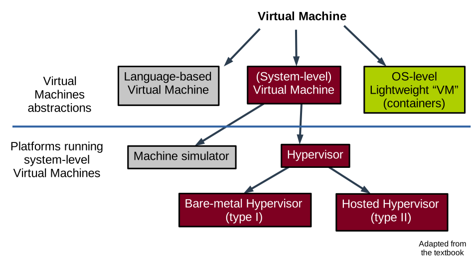
System-level Virtual Machines
System-level virtual machines create a model of the hardware for a (mostly) unmodified operating system to run on top of it.
Each VM running on the computer has its own copy of the virtualised hardware. This is the type of VM one creates when e.g., running two different OSes (here Linux and Windows) each within its own VirtualBox VM on a single physical machine:
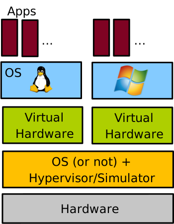
Machine Simulators and Emulators
Machine simulators and emulators create on a physical host machine a virtual machine of a different architecture. We already discussed emulation: it is useful for reasons of compatibility with legacy applications/hardware, software prototyping, etc. An example here would be to use QEMU in its full emulation mode.
Architecture simulators simulate computer hardware for analysis and study. This is useful for computer architecture prototyping, performance/power consumption analysis, research, etc. An example of a popular computer architecture simulator is Gem5. With emulation each guest instruction is interpreted in software, which is extremely slow: it is common to see 5x to 1000x slowdown when running in an emulated environment compared to native execution.
Hypervisor/VMM-based Virtual Machines
Contrary to emulation, a hypervisor-based VM creates a VM of the same architecture as the host. The hypervisor is also called Virtual Machine Monitor (VMM). This is the main type of VMs we will study in this course unit.
Hypervisor-based VMs rely on direct execution for performance reasons: the speed of software running in these VMs is very close to native execution. With direct execution, the VM code executes directly on the physical CPU, at a lower privilege level than the hypervisor, for security reasons that we will study in depth. A hypervisor still needs to rely on emulation for a very small subset of the instructions the guest executes: the VMM emulates only sensitive instructions. These are the instructions that would allow the VM to escape the VMM’s control if executed natively (e.g., installing a new page table). Upon encountering a sensitive instruction, the VM switches (traps) to the hypervisor which emulates it: trap-and-emulate model. Once the VMM is done emulating the sensitive instruction, the execution of the VM can resume directly on the CPU.
Examples of VMMs/hypervisors are Xen, Linux KVM, VMware ESXi, MS Hyper-V, Oracle VirtualBox, etc.
OS-level Lightweight “VMs”
OS-level lightweight sandboxing technologies create isolated environments that may look similar to a VM from the user’s point of view. However, there is no virtualisation of the hardware, and as such there is no virtual machine: all the isolation is managed by the host OS using mechanisms that restrict the view of OS resources for the software running within the sandbox environment. Containers represent a prime example of such lightweight OS-level virtualisation technologies. We will cover containers briefly in the last lecture of this course unit.
Hypervisors: Memory Denomination
We need to cover one last definition, related to how memory is organised in virtualised scenarios. For a non-virtualised machine, software running on the CPU executes load and store instructions to access memory. These load and store instructions target virtual addresses, and the MMU transparently maps these accesses to the corresponding physical memory based on the translation information contained in the page table currently in use. The page table is set up by the OS and is walked on every memory access to determine the target physical address.
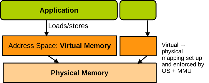
When running virtualised, we have something like this:
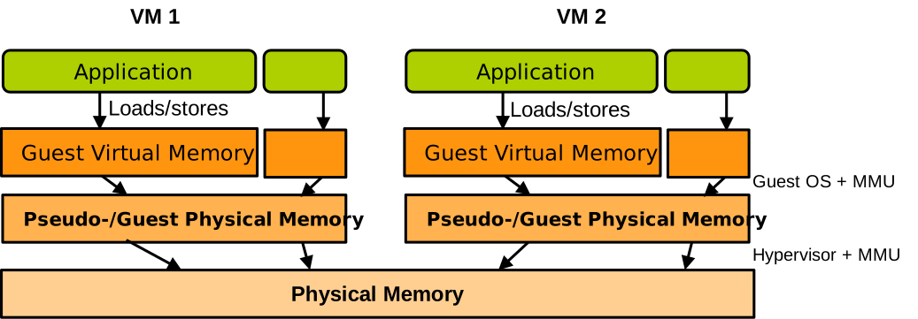
There is another level of translation added, which is taken care of by the hypervisor. It corresponds to the memory that the guest thinks is its physical memory. It is called pseudo physical memory or guest physical memory. Like virtual memory, it just corresponds to another level of indirection and does not hold any data – only physical memory does. So when software running in the VM accesses memory with load and store instructions, it targets virtual addresses – guest virtual addresses. The page table installed by the guest OS translates these accesses into guest physical memory accesses, and the hypervisor must somehow ensure that these guest physical memory accesses are translated into physical memory accesses. We will see how this is done soon.
The Theory of Virtualisation
You can access the slides 🖼️ for this lecture.
Here we’ll talk about how virtualisation works from the theoretical point of view. Why study the theory of virtualisation? First, it will help us understand the core requirements of virtualisation and the characteristics that an instruction set architecture (ISA) needs to have to be virtualisable. Second, it will allow us to understand the working principles of virtualisation on a hypothetical model of a processor that is much simpler than the CPUs we use today.
The Popek and Goldberg Theorem
We already mentioned this seminal virtualisation paper published in 1974 in Communications of the ACM:
Popek, Gerald J., and Robert P. Goldberg. “Formal requirements for virtualisable third generation architectures.” Comms. of the ACM 17.7 (1974): 412-421.
You can access the paper’s PDF by clicking on its picture above. It is well worth a read, in particular Sections 1 to 5. That being said, we’ll do a good summary of these sections here.
The original idea of the paper was to show that, at the time, some contemporary architectures were not virtualisable. Recall that by virtualisable here we mean that we want to be able to run several operating systems efficiently on the same machine. The authors take an at-the-time popular ISA as a case study: the DEC PDP-10, which was not virtualisable for a series of reasons defined in the paper.
To define the criteria an ISA must satisfy to be virtualisable, the paper starts by describing the key properties that a virtual machine monitor/hypervisor must present. These requirements are safety, equivalence, and performance. We’ll develop on these later. The paper then defines what is now known as the Popek and Goldberg Theorem, listing the requirements for an ISA to support such a VMM, i.e., to be virtualisable.
The paper did not attract much attention in the 1970s because virtualisation was not a popular topic. Later, as computers became much more common and widespread, there was a significant resurgence of interest in virtualisation. By the end of the 1990s, many actors were looking to run efficient virtual machines; however, the most popular ISA at the time, Intel x86-32, was not virtualisable: indeed, it did not satisfy the requirements pointed out in the paper by Popek and Goldberg. Following that, in the 2000s, when the 64-bit instruction sets (e.g., x86-64 or ARM64) that we use today were created, their designers took great care to follow the principles defined in the paper. And they succeeded, as on these ISAs we can run virtual machines very efficiently.
By studying this paper, we will also learn about the working principles of virtualisation and how a virtual machine monitor works when it runs on a virtualisable ISA. We will explain the theorem as follows. We’ll first describe the simplified model of processor presented in the paper, and will then present how a regular operating system would run without virtualisation on top of that processor model. Next, we will present the Popek and Goldberg theorem, which lists the characteristics that an ISA needs to have to be virtualisable. Then we will describe how our simplified CPU model can be virtualised and how a virtual machine monitor would work on that CPU. Finally, we will briefly give examples of ISAs that do not satisfy the theorem, and we’ll see how they cannot be virtualised concretely.
Simplified CPU Model
Hardware Mechanics
This processor has two privilege levels: user and supervisor.
The physical memory it can access is contiguous, starts at address 0 and is of size SZ.
Virtual memory is supported and an application running on the CPU accesses the virtual address space with loads and stores which are mapped to physical memory by the MMU.
Virtual memory is implemented through segmentation (remember this paper is very old): at any time the virtual address space seen by what is running on the CPU ranges from virtual address 0 to virtual address L, and it is mapped to a segment of physical memory from physical address B to physical address B + L.
This is illustrated here:
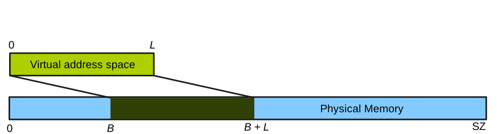
The CPU state is composed of 4 control registers that together form the Processor Status Word (PSW). The control registers are as follows:
- The current privilege level
M(for mode), which can take the valueSfor supervisor mode, orUfor user mode. - The segment register (
B,L): as mentioned previously, these give the base address of the currently mapped segment and its length. - The program counter that points in virtual memory to the current instruction being executed.
A complete view of our processor so far is as follows:
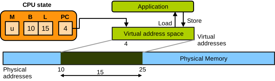
We also need CPU support for entering the OS following an interrupt or exception.
This is also called a trap.
It works as follows.
Assume the CPU runs an application in user mode.
There is a trap, for example because the application is making a system call.
The PSW at that stage represents the CPU state for the application, and it needs to be saved somewhere in memory.
There is a dedicated space for that, it’s the first slot in memory MEM[0].
We also need to switch to the kernel, so we load the kernel CPU state that was previously saved in another dedicated location, MEM[1].
This kernel state loads the kernel memory segment which simply gives the OS access to the entire physical memory, and sets the program counter to a predefined kernel code location which is the trap entry point.
Of course the privilege level of the kernel PSW is set to supervisor mode.
When this is done the kernel starts to run and processes the trap:
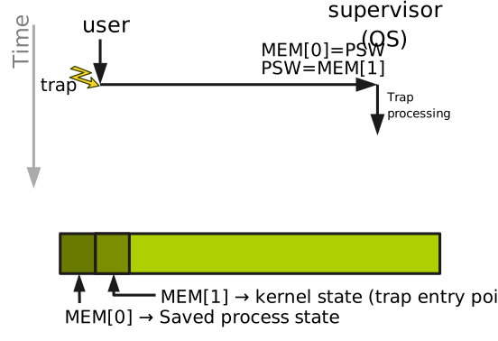
When the kernel is done processing the trap, to return to user space the PSW is loaded with the previously-saved application CPU state from MEM[0].
The application can then resume:
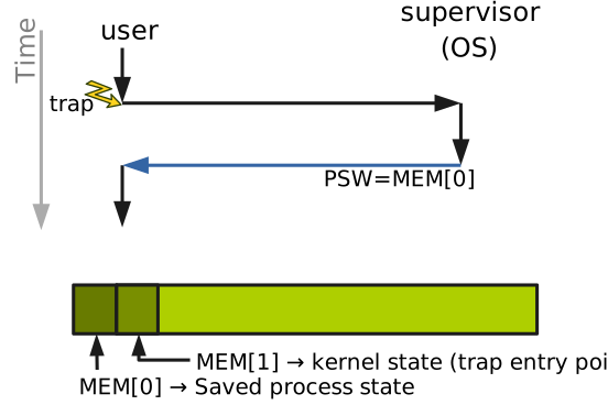
Non-Virtualised OS Operation
When running software without virtualisation, the OS kernel runs in supervisor mode (M = s) and applications run in user mode (M = u).
When it boots, the kernel loads MEM[1] with the kernel state that the CPU should take upon a trap: M:s, B:0, L:SZ, PC:trap_entry_point.
That is: supervisor privilege level, access to all physical memory with B = 0 and L = SZ, and the program counter set to the trap entry point in the kernel code.
For each application, the kernel allocates a contiguous range of physical memory defined by (B, L).
For security reasons, the kernel ensures that the segments given to applications do not overlap.
The kernel launches and resumes an application whose address space is defined by segment [B, B+L] and which wants to run the instruction pointed to by PC by loading its PSW with the following values: (M:u, B:B, L:L, PC:PC).
Finally, when the kernel runs after a trap, it decodes the application instruction that caused the trap and takes action.
The Popek and Goldberg Theorem
Hypervisor Objectives and Requirements
Back to the paper, the authors ask the following research question: what are the requirements for building a hypervisor for that CPU in such a way that the hypervisor:
- can execute one or more virtual machines;
- can support any operating system designed to run non-virtualised for that CPU;
- supports arbitrary, unmodified, and potentially malicious guest OSes designed for the same architecture;
- is in complete control of the hardware at all times; and
- is efficient and shows at worst a small performance decrease versus non-virtualised execution?
To reach these objectives, the hypervisor needs to comply with the following three fundamental requirements:
-
Safety: the VMM must be in complete control of the hardware at all times. It should not assume that guest code (guest applications and the OS) will behave correctly; in fact, it should assume the guest can be malicious. For that reason, the VMM must enforce isolation between a VM and the VMM/hardware, and between VMs themselves.
-
Equivalence: a VM should be a duplicate of the physical hardware, and the guest OS and its applications should not have to be modified to run in a VM. Their behaviour in a VM should be exactly the same as if they were running natively.
-
Performance: when running virtualised, the guest OS and its applications should see a minimal performance slowdown compared to native, non-virtualised, execution.
To satisfy the performance criteria we want to run as many guest instructions as possible directly on the CPU. However, to satisfy the safety criteria we want to make sure that any guest instructions that may allow the guest to escape the virtualisation isolation will trap to the hypervisor. This way the hypervisor can emulate that instruction safely without breaking the isolation between VMs and itself. Hence, the central idea behind constructing an efficient and secure hypervisor is to run the hypervisor in supervisor mode and run the guest applications and the guest OS in user mode. The hope is that every instruction that would allow a guest to escape the isolation enforced by the hypervisor would be forbidden in user mode hence if a guest attempts to execute such instructions they would trap to the hypervisor to be emulated.
This is not doable with every architecture; what we’ll present next will tell us the properties an ISA should have so that we can build such a virtual machine monitor on that ISA.
Classifying Instructions
The last thing we need before presenting the theorem is to classify instructions.
The first category is called sensitive instructions. It is subdivided into two subcategories:
-
Control-sensitive instructions: these are the instructions that update the system state, for example the instructions modifying the PSW in our example, or
LGDTon Intel x86-32 which allows installing new interrupt handlers. -
Behaviour-sensitive instructions: these are the instructions whose semantics depends on the value of the system state such as the privilege level. An example here is
POPFon x86-32 that loads a status register with data from the stack: it works fine in supervisor mode (ring 0) but fails silently in user mode (ring 3).
The instructions that are not sensitive are called innocuous instructions: they do not update the system state, and their behaviour does not depend on it either.
A second category of instructions is privileged instructions.
We already covered these in a previous lecture: they can only be executed in supervisor mode and trap when executed in user mode.
An example of such instruction is HLT, that shuts down the CPU in supervisor mode but traps if executed in user mode on x86-32.
Instructions can be privileged or not independently of their sensitive/innocuous nature.
The Theorem
We can now state the Popek and Goldberg theorem, which specifies the requirements for an instruction set to be virtualisable:
For a given ISA, a VMM may be constructed if the set of sensitive instructions for that ISA is a subset of the set of privileged instructions, i.e.
if {control-sensitive} ∪ {behaviour-sensitive} ⊆ {privileged}
The theorem simply states that for a given ISA to be virtualisable, the set of all sensitive instructions needs to be a subset of the privileged instructions. In other words, every sensitive instruction must trap when executed in user mode.
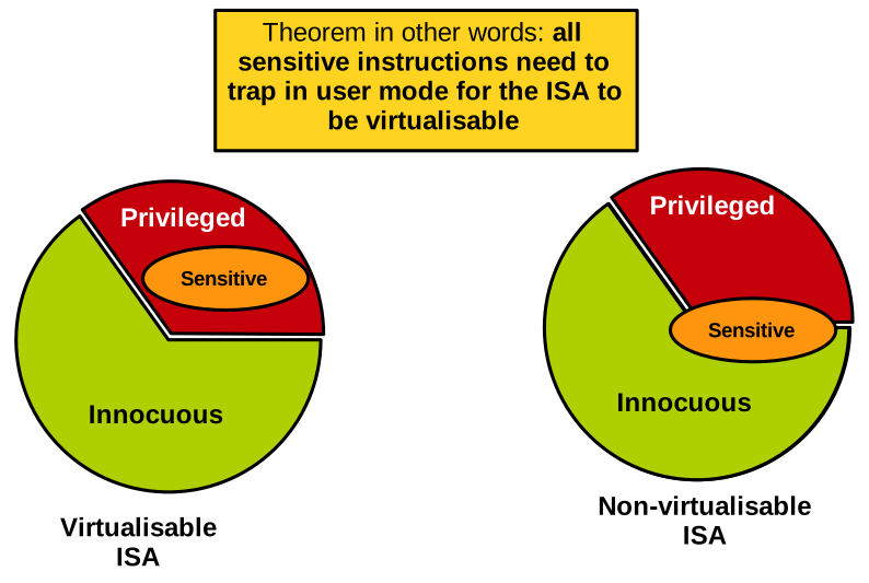
In the diagram above, we can see a virtualisable ISA on the left, satisfying the theorem requirement. On the right we have a non-virtualisable ISA: a subset of sensitive instructions is not privileged and will not trap when executed in user mode.
So why can’t an ISA be virtualised if some of its sensitive instructions do not trap when executed in user mode? Recall that with the hypervisor we want to build, both guest applications and the guest OS run in user mode. If you consider a control-sensitive instruction that would not trap in user mode, any guest could update the state of the system without supervision from the hypervisor. Imagine a guest being able to install an arbitrary segment register or page table, and map physical memory it is not supposed to access. That would break the safety criteria the hypervisor needs to maintain, and things would not work. If you now consider a behaviour-sensitive instruction that does not trap in user mode, it means that the guest OS, when executing this instruction and expecting the supervisor mode behaviour, will actually see the user mode behaviour: this breaks the equivalence criteria the hypervisor needs to maintain, and once again things do not work.
Hypervisor Operation
Basic Principles
Let us now discuss how a hypervisor that satisfies the Popek and Goldberg requirements would work, with the goal of reaching the safety, equivalence, and performance objectives. The VMM operates as follows: for performance reasons, we want to run as much guest code as possible directly on the CPU without trapping. So, as we mentioned, the hypervisor will run in supervisor mode, and the guest—including its operating system—will run in user mode:
The hypervisor will reserve some contiguous memory for itself.
That memory should never be accessed by the guest for obvious security reasons.
The hypervisor will also allocate contiguous ranges of physical memory, one for each VM.
We can define each VM range with a base physical address addr0, and a length, memsize:
For each VM, the hypervisor keeps in memory a data structure that represents a software model of what the VM thinks is the current PSW.
We call it the virtual PSW, vPSW.
It has the same registers as the real PSW: a privilege level M, which is user when the VM runs an application and supervisor when the guest OS runs; a segment register (B, L) representing the address space of what is currently running in the VM; and a program counter PC.
This can be illustrated as follows:
Starting and Resuming a VM
When starting a VM or resuming execution following a trap, the hypervisor loads the real PSW as follows:
- As explained previously, the real privilege level of a VM is always user mode:
M’ ← u. - The real segment base address is the base address of the physical memory allocated to the VM,
addr0, plus the base address of the vPSW,vPSW.B, i.e.B’ ← addr0 + vPSW.B. - The real segment length is the vPSW length:
L’ ← vPSW.L. - The real program counter is that indicated in the vPSW:
PC’ ← vPSW.PC.
The hypervisor resuming a VM in the state presented on the last diagram can be illustrated as follows:
For security reasons, addresses from the vPSW are checked by the hypervisor before being loaded into the real PSW so that we do not load into the real PSW anything that would go beyond the limits of what is allocated to the VM.
Further, any attempt by the guest to modify M, B or L will trap: the theorem hypothesis assumes all control-sensitive instructions are also privileged.
Because the guest always runs in user mode (independently of the value of vPSW.M), it will trap when the guest OS attempts to use them.
Hence, the hypervisor can maintain correct values for the vPSW, as it needs to always keep track of what the VM thinks the PSW is.
Handling Traps
When the VM traps, the hypervisor keeps the vPSW up to date by writing the trap’s PC into it: vPSW.PC ← PSW.PC.
Based on the instruction that caused the trap, the VMM will emulate a non-virtualised machine’s behaviour.
What to do depends on what the guest was running when it trapped: application code, or kernel code?
If the guest kernel caused the trap (vPSW.M is s), it means the guest OS probably executed a sensitive instruction.
The VMM handles that depending on the instruction in question.
For example, if the guest is trying to update the segment register, the vPSW is updated with what the guest wants to write in there.
When we return to the guest from the trap, the real PSW will be updated with the method we just described.
This way the MMU is configured differently from what the guest requests, but this is also completely transparent from the guest’s point of view.
Before returning to the guest, the VMM will set the vPSW’s PC to the next instruction to denote the fact that the emulated instruction ran successfully.
Upon a trap happening while the guest was running application code (vPSW.M is u), the application is either making a system call or experiencing a fault such as a division by zero.
To manage that fault, the guest OS needs to run: the hypervisor needs to emulate a transition to the guest OS.
The hypervisor starts by saving the guest application’s state (which is the vPSW’s value) inside the VM’s memory at the dedicated location, which is the VM’s equivalent of MEM[0].
Then it loads into the vPSW the guest OS state from the guest’s memory equivalent of MEM[1].
Finally, it loads the real PSW based on the method we presented previously to resume the VM and start executing its kernel.
This can be illustrated as follows:
On this diagram the vPSW is a data structure present somewhere in the hypervisor’s memory in red.
It is copied in the VM’s MEM[0] (step 1) to emulate saving the state of the application that was running in the VM.
The guest OS’ state is loaded in the vPSW from the VM’s MEM[1] (step 2).
The vPSW will then be restored into the hardware PSW as previously described.
Theorem Violations
Going back to the theorem, because all guest control-sensitive instructions that update the state of the system trap to the hypervisor, the hypervisor can check them, for example to make sure a VM does not map memory outside of what it can access. The hypervisor can also emulate them, to give each VM the illusion that it is in total control of the hardware, as it would be when running natively.
The transition instructions between the guest application and kernel need to trap to the hypervisor, so that it can update the mode register of the vPSW. This way the hypervisor knows when a trap originates from the guest kernel or application, and it can emulate it accordingly. Transition instructions are sensitive, so they will trap. Behaviour-sensitive instructions, for example reading the values of the PSW, will also trap. Once again the real PSW is loaded with values that are different from what the guest OS thinks is in the PSW. So if the guest OS tries to read these registers, the hypervisor will return the emulated values, so we can maintain equivalence.
Many ISAs proposed between the 1970s and 2000s violated the theorem and were not virtualisable properly.
A prime example here is x86-32, which had POPF, a behaviour-sensitive instruction that did not trap but rather failed silently when executed in user mode.
When executed in supervisor mode, this instruction was used by the OS to query important information about interrupts.
So, assuming an x86-32 virtualised guest OS running in user mode, these queries would fail silently, and the OS would misbehave by acting on garbage interrupt information.
This was a problem because the demand for virtualisation became quite high at that time when x86-32 was the most popular ISA.
Another example of theorem violation was the DEC PDP-10, which had a JRST1 instruction performing a world switch that returns to user mode from supervisor mode.
That instruction would not trap when run in user mode, hence with a virtualised guest OS the hypervisor would be unable to catch it to keep track of the mode the VM thinks it is running in (user/supervisor).
Because of a growing need for virtualisation by the end of the 1990s/early 2000s, techniques were developed to try to virtualise ISAs violating the theorem. Each of them had to compromise on some of the key objectives of virtualisation. For example, introducing more emulation by running the entire guest OS or at least every access to the guest page table as emulated would allow virtualising x86-32, but it was very slow, breaking performance. Another approach was paravirtualisation, where the guest OS was modified to be virtualisation-aware (e.g. not to issue any of the sensitive instructions that did not trap in user mode), breaking equivalence. Overall, it was OK to compromise on performance or equivalence, but of course never on safety.
CPU & Memory Virtualisation
You can access the slides 🖼️ for this lecture.
Introduction
We have seen that x86-32, among other ISAs, was not virtualisable based on the Popek and Goldberg theorem. And that attempts at virtualising it had to compromise on performance or equivalence. Due to the high demand for virtualisation in the early 2000s, and the related problems with x86-32, the next-generation ISA, x86-64 (first proposed in the early 2000s), did not make the same mistake. x86-64 was designed with hardware-based virtualisation support in mind. This is achieved with Intel processors using three key technologies: VT-x for CPU virtualisation, Extended Page Tables (EPT) for memory virtualisation, and VT-d for I/O virtualisation. We will focus on Intel here, but note that AMD, a manufacturer of x86-64 CPUs, has very similar technologies.
x86-64 CPU Virtualisation with VT-x
Motivation
Let us start with CPU virtualisation. The existing software techniques used to virtualise x86-32 had the following challenges. First, the guest OS runs in a privilege level it was not designed for, namely user mode. With x86, privilege levels are called rings. Supervisor mode is ring 0 and user mode is ring 3. Yet we have guest OSes running in ring 3 for virtualisation, whereas they were designed to run in ring 0. Second, the hypervisor needs to be located somewhere in memory and be inaccessible from the guests. Third, the performance impact of the traps, necessary to emulate every sensitive operation, is significant. The traps representing guest-host transitions are frequent and costly, leading to significant performance slowdowns.
The key design idea behind VT-x, x86-64’s hardware support for CPU virtualisation, was to propose a holistic solution rather than addressing each issue with x86-32 separately.
For example, changing the semantics of individual instructions such as POPF would be detrimental to backward compatibility.
The x86-64 designers instead addressed all issues by introducing a new mode of execution.
The entire CPU state is duplicated into two modes: root mode for running the hypervisor and host operating system code, and non-root mode for virtual machine code.
VT-x Overview
The two modes are illustrated here: a diagram showing a machine with one hypervisor and host OS running in root mode at ring 0, and host-level applications running in root mode at ring 3. We also have two VMs, each running a guest OS in non-root mode in ring 0, and guest applications in non-root mode in ring 3.
At any point in time the CPU is either in root or non-root mode, and privilege levels (rings) are orthogonal to the root/non-root modes and are available in both. Each mode has its own address space, which is switched automatically upon transitions, including virtual memory translation caches. This allows the hypervisor and other host-level software to be well isolated from the guest software.
VT-x and P&G
Remember the key objectives for a proper hypervisor that we listed in the previous lecture. In terms of equivalence, the state of the virtualised CPU exposed by VT-x in non-root mode to VMs is an exact duplicate of the physical CPU state: guests can run x86-64 code and are also backward compatible with x86-32. Regarding safety, with architectural support the hypervisor codebase is much simpler, which leads to a reduced attack surface compared to approaches based on emulating the execution of the entire guest OS or on paravirtualisation, which need to maintain complex invariants. Finally, concerning performance, it was not a primary goal at first: the first generation VT-x CPUs were actually slower than state-of-the-art paravirtualised/OS emulation approaches.
With the root and non-root modes introduced in x86-64, we can rework the Popek and Goldberg theorem as follows:
When executed in non-root mode, all sensitive instructions must either 1) cause a trap or 2) be implemented by the CPU and operate on the non-root duplicate of the CPU state
If each sensitive instruction traps to the VMM in root mode, it would satisfy the equivalence and safety criteria. However, these traps are very costly, and we cannot have them be too frequent. Ideally we want as few traps as possible to keep performance close to native execution. Clearly, managing the virtualisation of more privileged instructions in hardware means implementing more logic in the CPU, so there is a trade-off between hardware complexity and cost versus performance here.
Root/Non-Root Transitions
Let us briefly see how VT-x manages transitions between root and non-root modes.
Assume the hypervisor is initially running in root mode.
The hypervisor can start and resume a VM with the VMLAUNCH and VMRESUME instructions.
This causes the CPU to switch to non-root mode and start running the guest.
Conversely, transitions from the VM to the hypervisor are called VM exits.
The VM will transition to the hypervisor following a trap or an explicit call to switch to the hypervisor via the VMCALL instruction.
In these cases the CPU switches from non-root to root mode and starts running hypervisor code to handle the trap.
When a VM exit occurs, the CPU maintains a data structure containing information about the guest, such as the reason for the VM exit.
This is called the Virtual Machine Control Structure (VMCS).
The hypervisor must use specific instructions to access it: VMREAD and VMWRITE.
These operations and the VMCS can be illustrated as follows:
The list of categories of VM exit reasons follows:
| Category | Description |
|---|---|
| Exception | Guest instruction caused an exception (e.g. division by 0) |
| Interrupt | Interrupt from I/O device received during guest execution |
| Triple fault | Guest triple faulted |
| Root-mode sensitive | x86 privileged/sensitive instructions |
| Hypercall | Explicit call to hypervisor through VMCALL |
| I/O | x86 I/O instructions, e.g. IN/OUT |
| EPT | Memory virtualisation violations/misconfigurations |
| Legacy emulation | Instruction not implemented in non-root mode |
| VT-x new | ISA extension to control non-root execution (VMRESUME, etc.) |
VM exits occur when the CPU faults or invokes a system call (software exceptions), when an interrupt is received from an I/O device, when the guest encounters a triple fault, or when it invokes a sensitive instruction. The guest can also voluntarily trigger a VM exit, which is called a hypercall. The hypercall is to a hypervisor what a system call is to an operating system. Other categories include I/O instructions, memory virtualisation VM exits, instructions that need to be emulated, and VT-x instructions themselves.
Introduction to KVM
KVM is a hypervisor integrated into the Linux kernel and leveraging VT-x on x86-64. KVM stands for Kernel-based Virtual Machine. It is a type 2 hypervisor designed within Linux from the ground up assuming hardware support for virtualisation, like VT-x for x86-64 and equivalent technologies for the other modern ISAs.
KVM is a module in the Linux kernel code, so it lives in kernel space. KVM partially manages virtual machines by handling traps, maintaining the Virtual Machine Control Structure (VMCS), and so on. Still, KVM must also rely on a user-space program to handle other virtual machine management tasks, in particular resource allocation. That user-space program is very often QEMU. QEMU was originally a machine emulator, but CPU and memory emulation can be disabled when running on top of KVM, because they are managed by VT-x and the memory virtualisation technology we will cover shortly: this makes things much faster, close to native performance. The KVM + QEMU combination is arguably the most popular hypervisor today.
x86-64 MMU Virtualisation with EPT
We have covered the CPU; let us now discuss hardware-assisted memory virtualisation for x86-64. The first iterations of x86-64 did not have support for hardware-assisted memory virtualisation, only VT-x for the CPU. They assumed disjoint page tables for root and non-root modes, which was efficient to isolate the hypervisor from the guest by making sure they could not map each other. However, every guest page table update still needed to trap to the hypervisor to be validated, to make sure the guest does not try to map something it should not have access to. This is called shadow paging, and it is notoriously slow because page table updates are quite frequent.
Without hardware support for MMU virtualisation, another option is paravirtualisation, i.e., to modify the guest so that it does not update page tables directly, but rather requests the hypervisor to do so in a controlled fashion. As we saw, paravirtualisation breaks equivalence, so this solution is not ideal either.
Extended Page Tables: Introduction
There was a need for hardware support for memory virtualisation, similar to what VT-x does for the CPU. The technology for memory virtualisation is called Extended Page Tables and was presented in this seminal paper in 2008:
R. Bhargava et al., Accelerating Two-Dimensional Page Walks for Virtualised Systems, ASPLOS’08
With EPT the guest OS maintains its page tables normally. It can update them freely without traps to the hypervisor. There is one page table per guest process, and it maps guest virtual to guest pseudo-physical addresses. The key idea behind EPT is to add a second level of address translation, the extended page table. There is one extended page table per VM, and it maps guest pseudo-physical addresses to host physical addresses:
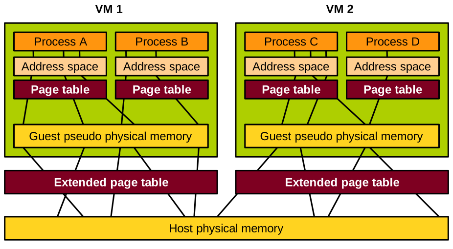
The hypervisor is in total control of these extended page tables, hence it can ensure that guest OSes map only the memory they are allowed to access.
With performance in mind, having to walk 2 levels of page table is concerning. Still, EPT is designed such that the translation caches, i.e. Translation Lookaside Buffers (TLBs), will cache the guest virtual to host physical mapping directly. Knowing that the TLB hit rate is about 95% in modern CPUs, there is no need to walk two levels of page tables for the majority of VM memory accesses. However, if there is a TLB miss, then these two levels must be walked: the guest’s page table, and the extended page table.
EPT Walk
Before explaining the EPT walk, let us see how the MMU walks a traditional (non-virtualised) page table to perform address translation on a memory access.
The page table is rooted in the %cr3 register.
Different parts of the target virtual address will index each level of the page table
until the target data page is found.
An offset from the beginning of that page, derived from the least significant bits of the address, is added to find the target byte to load or store.
This is illustrated here:
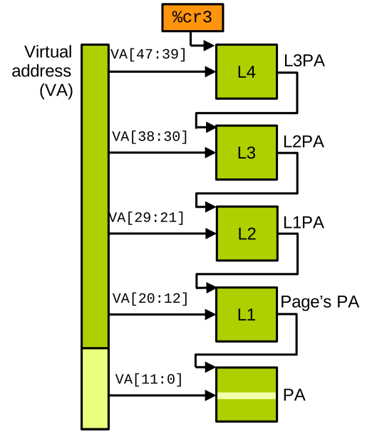
On the left is the virtual address the CPU wants to access, and on the right is the page table. The goal of the page table walk is to find the physical address corresponding to the virtual one, in order to perform the memory access.
The %cr3 register contains the physical address of a page constituting the root of the page table.
On standard CPUs page tables are a tree with 4 levels, and the root is the 4th level.
That address contains 512 64-bit entries, each of which is a pointer to a page in the next (3rd) level of the page table.
The root of the page table is indexed by bits 39 to 47 of the virtual address the CPU wants to access (note that most modern CPUs do not use the full 64 bits of a virtual address, but rather 48).
This selects an entry in the root page, indicating which 3rd level page to use next.
The bits 30 to 38 of the address are used to index that page, giving us the 2nd level page, indexed with bits 21 to 29, giving us the 1st level page, indexed with bits 12 to 20.
The 1st level page table entry points to the page containing the physical address we need, and that page is finally indexed with bits 0 to 11 to find the target byte.
When running virtualised, address translation must walk both the guest page table and the extended page table. Things work as follows:
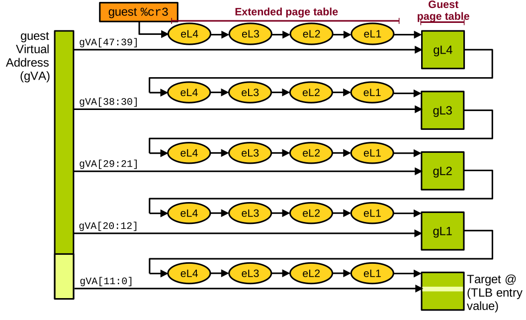
We have the virtual address targeted by the guest on the left.
The guest page table is rooted in %cr3.
It contains a guest pseudo-physical address, so we first need to translate it into a host physical address.
We therefore walk the extended page table to figure out which physical page contains the root of the page table, which is level 4.
Once found, it can be indexed with the most significant bits (bits 39 to 47) of the target address, which gives us the address of the next-level page (3rd level).
However, that address is a guest pseudo-physical address, and we need to similarly translate it into a host physical one, so we walk the extended page table again.
This process repeats to find the 2nd level page, the 1st level page, and finally the target data page, which can be indexed by the least significant bits (0 to 11) of the target guest virtual address to find the byte the guest wants to load or store.
In the end, to walk the 2D page table, we had to do 24 memory accesses to load or store a single byte. By comparison, only 4 memory accesses are needed to walk a standard page table when running non-virtualised. That is a very high overhead, but remember that 95% of guest memory accesses do not need to go through this, as they hit in the translation cache (the TLB – Translation Lookaside Buffer).
Memory Virtualisation in KVM
KVM of course makes use of extended page tables to manage the VMs’ memory. Address translation works as follows:
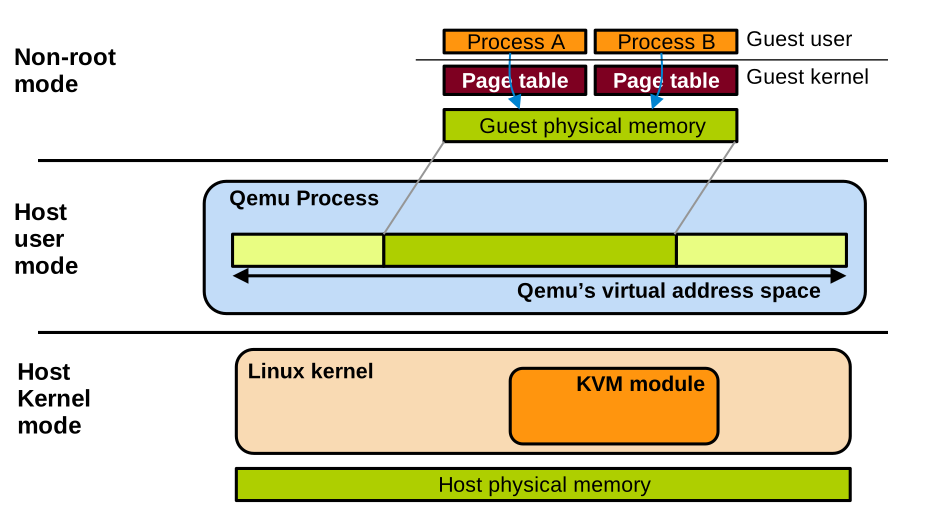
The guest manages its own page tables, one per guest process, with minimal intervention from KVM.
QEMU lives in the host user space as a regular process.
Like every other process, it has its own virtual address space.
QEMU makes a large call to malloc to allocate a large contiguous buffer that will be the guest’s pseudo-physical memory.
The KVM module lives in the host kernel. It sets up and manages the extended page tables that map the guest pseudo-physical addresses to host physical memory.
Sometimes the QEMU process needs to read and write the VM’s memory too, for example when virtualising I/O as we will see next. For this, it can read and write in that large area of virtual memory it allocated for the VM, and the page tables of QEMU on the host will be used for the translation, as with any other host process.
I/O Virtualisation
You can access the slides 🖼️ for this lecture.
After we covered how CPU and memory are virtualised on modern ISAs, let’s now talk about I/O virtualisation.
I/O Interposition
Similar to CPU and memory virtualisation, the first attempts at virtualising I/O were achieved in software without hardware support. This is called I/O interposition. The hypervisor creates a software model of a virtual I/O device, which the guest OS will access using a driver, as if the device were a real, physical one. The hypervisor is also in charge of connecting the virtual device to the real devices on the host to actually perform I/O such as accessing the filesystem or the network.
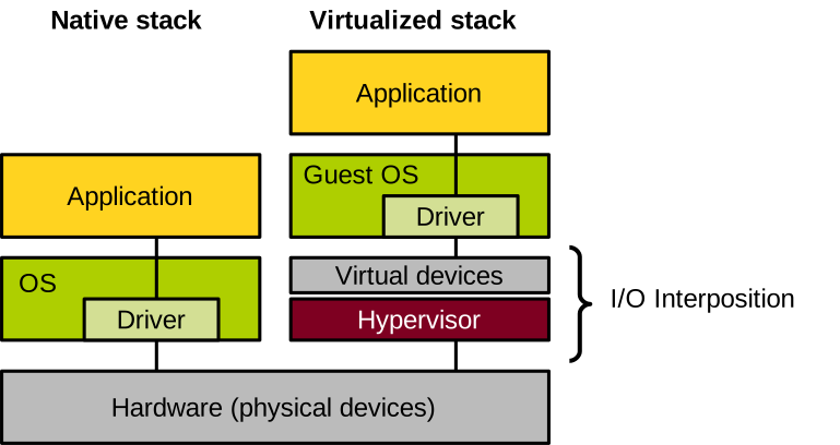
Virtualising devices this way has many benefits. One is device consolidation: we can create many virtual devices on top of a smaller number of physical devices. For example, you can have a host with a single hard disk running several virtual machines, each with its own virtual disk. This helps reduce cost and increases device utilisation. Conversely, several physical devices can also be aggregated into a single virtual one, in order to achieve higher throughput or better reliability (e.g. through data redundancy). Because the virtual device is implemented in software, it is easy for the hypervisor to capture its state at a given point in time: this is quite useful to enable features such as virtual machine suspend/resume or migration, including between hosts equipped with different models of physical devices. Finally, device virtualisation can also enable features that are not normally supported by physical devices, for example taking disk snapshots, compressing or encrypting I/O, etc.
Physical I/O
Before diving into virtual I/O, let’s briefly talk about how I/O works on a non-virtualised machine. Overall, there are three ways for the system and devices to interact:
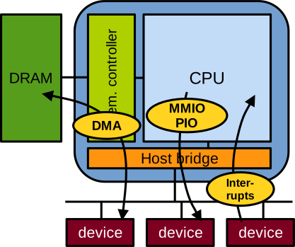
First, port-based or memory-mapped I/O (MMIO). With this method, device registers are mapped somewhere in the address space, and when these addresses are read or written, the CPU actually communicates with the device, reading from or writing to the device’s registers. This method of communication is unidirectional, from the CPU to the device, and can only transmit very small register-sized messages. For example, when the CPU configures the network card to enable networking, this is done through memory-mapped I/O.
Second, interrupts: these are unidirectional signals sent from the device to the CPU. Interrupts are a form of notification; they do not carry data. For example, when the network card wants to notify the CPU that a packet has been received and should be fetched, it uses an interrupt.
Third, direct memory access (DMA): it is bidirectional, and is used to transfer large quantities of data between memory and the device. For example, when the CPU needs to send data to the network or receive data from the network through the network card, it uses DMA.
Large DMA data transfers between memory and I/O devices are realised with the use of ring buffers in memory. A ring buffer is a producer-consumer system, generally enabling unidirectional communication. To establish such communication, the CPU configures the device using memory-mapped I/O and specifies, in some of the device’s control registers, information about the ring buffer: what its base address and length are, and where the head and tail pointers are located.
For CPU-to-device transfers, the device consumes data from the head pointer and updates it:
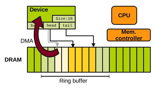
The CPU produces data at the tail pointer, updating it too:
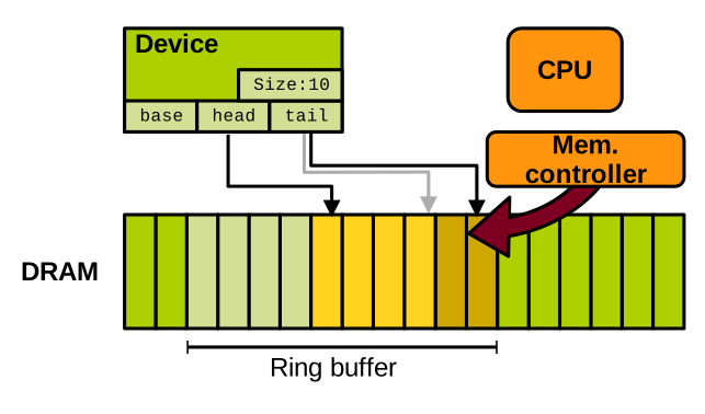
Because memory is shared between the device and the CPU, they need to synchronise. Memory-mapped I/O is used for CPU-to-device synchronisation, for example to signal the start of a DMA transfer. Interrupts are used for device-to-CPU synchronisation, for example to notify the end of a DMA transfer.
I/O Virtualisation without Hardware Support
Let’s now see how this can be virtualised, first entirely in software without hardware support.
Device Emulation
A first technique is I/O emulation. We have seen that the interface between the OS and devices is quite simple. The OS discovers and controls devices with memory-mapped I/O, and devices respond with interrupts and DMA. The hypervisor can create a virtual device that entirely emulates the behaviour of a device behind the same interface exposed to the guest OS. Of course, every I/O-related action performed by the guest OS must trap. Memory-mapped I/O involves sensitive instructions, so it will indeed trap. The hypervisor also needs to map DMA memory as inaccessible so that any access will trap. Concerning device-to-CPU notification, the hypervisor can also emulate it by injecting interrupts into the guest. This is done by calling the handlers registered by the guest in the virtual interrupt controller, which is also handled by the hypervisor. Finally, to emulate DMA, the hypervisor can simply read from and write to the relevant guest memory areas.
With KVM and Qemu, the hypervisor uses one thread for each virtual core of the VM; we call these virtual CPUs, or vCPUs. It also creates one thread for each virtual device. Here is an illustration of a VM with two virtual cores and two virtual devices:
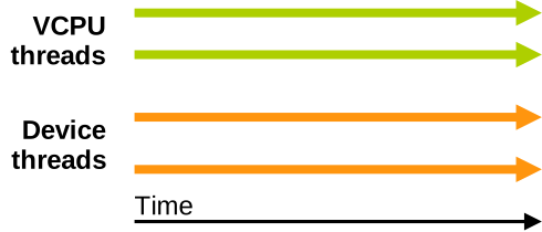
Assume the VM is running and one of the cores wants to perform I/O. As illustrated below, it initiates memory-mapped I/O communication with the virtual device. This will trap to the hypervisor, which will defer the handling of that I/O to the thread managing the virtual device. Assuming this is a long operation, such as a DMA transfer, the guest will resume after the transfer starts, and the hypervisor will inject an interrupt later when the transfer is done. This mimics exactly what happens with a real device.
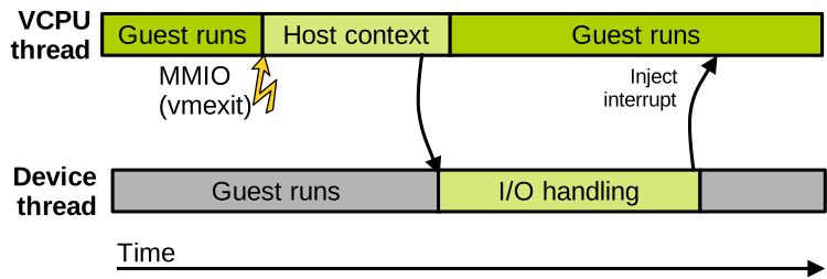
The following is an example of the lspci output on a standard Linux Qemu/KVM machine:
00:00.0 Host bridge: Intel Corporation 440FX - 82441FX PMC [Natoma] (rev 02)
00:01.0 ISA bridge: Intel Corporation 82371SB PIIX3 ISA [Natoma/Triton II]
00:01.1 IDE interface: Intel Corporation 82371SB PIIX3 IDE [Natoma/Triton II]
00:01.3 Bridge: Intel Corporation 82371AB/EB/MB PIIX4 ACPI (rev 03)
00:02.0 VGA compatible controller: Device 1234:1111 (rev 02)
*00:03.0 Ethernet controller: Intel Corporation 82540EM Gigabit Ethernet Controller (rev 03)
*00:04.0 Ethernet controller: Red Hat, Inc Virtio network device
00:05.0 Communication controller: Red Hat, Inc Virtio console
You can see two network cards in this list: the first, the Intel one, is a fully emulated device, working as we just described. The second, the Virtio one, is called a paravirtualised device. We will discuss this type of device virtualisation in more detail shortly.
Looking more closely at the Intel (fully emulated) network card, we can see the memory address where the memory-mapped I/O registers are located: 0xfebc0000.
00:03.0 Ethernet controller: Intel Corporation 82540EM Gigabit Ethernet Controller (rev 03)
    Subsystem: Red Hat, Inc QEMU Virtual Machine
    Physical Slot: 3
    Flags: bus master, fast devsel, latency 0, IRQ 11
    Memory at febc0000 (32-bit, non-prefetchable) [size=128K]
    I/O ports at c000 [size=64]
    Expansion ROM at feb40000 [disabled] [size=256K]
    Kernel driver in use: e1000
    Kernel modules: e1000
We can also see the name of the driver used for that virtual device: e1000. This model of network card is quite old but also widespread, so most OSes already have a driver for it, ensuring good compatibility. The data sheet for the physical version of this Intel network card lists the memory-mapped I/O registers exposed to the OS for communication:
| Category | Name | Full name | Offset | Description |
|---|---|---|---|---|
| Receive | RDBAH | Receive descriptor base address | 0x02800 | Base address of Rx ring |
| Receive | RDLEN | Receive descriptor length | 0x02808 | Rx ring size |
| Receive | RDH | Receive descriptor head | 0x02810 | Pointer to head of Rx ring |
| Receive | RDT | Receive descriptor tail | 0x02818 | Pointer to tail of Rx ring |
| Transmit | TDBAH | Transmit descriptor base address | 0x03800 | Base address of Tx ring |
| … | … | … | … | … |
| Other | STATUS | Status | 0x00008 | Current device status |
| Other | ICR | Interrupt cause read | 0x000C0 | Cause of the last interrupt |
| … | … | … | … | … |
Each register is accessible by reading from or writing to a particular location in memory, at a given offset from the base address where these registers are mapped.
Each register also serves a particular purpose: setting up ring buffers for DMA, indicating the status of the device, the cause of the last interrupt, etc.
For example, to read the cause of the last interrupt (the ICR register), the driver running on the CPU reads at the physical address base + offset: 0xfebc0000 + 0xc0 = 0xfebc00c0.
What the device does upon receiving this command is documented in the device’s data sheet.
The emulated model for this device, as implemented in Qemu, mimics exactly the behaviour of the real network card when each of these registers is read or written by the virtual machine.
With Qemu/KVM, each interaction with the emulated e1000 NIC’s memory-mapped registers traps to KVM first, which redirects I/O management to Qemu. The code implemented by Qemu for emulating the Intel network card can be found here. It is not very large, at less than two thousand lines of code. The following excerpt shows the code executed when the VM reads the memory-mapped register that holds the cause of the last interrupt:
static uint32_t mac_icr_read(E1000State *s, int index)
{
    uint32_t ret = s->mac_reg[ICR];

    set_interrupt_cause(s, 0, 0);
    return ret;
}
As you can see, that information is held in a data structure and is returned to the VM by the emulation code, in effect mimicking in software the behaviour of a hardware NIC.
I/O Paravirtualisation
Full emulation is great for compatibility, because we are emulating real devices for which we know existing guest OSes will have the drivers. However, these real devices have never been designed with virtualisation in mind. For that reason, communication between the VM and the emulated device involves a lot of VM exits, which are quite costly and hurt performance. I/O paravirtualisation is an alternative approach, in which the relevant virtual devices are designed entirely with virtualisation in mind. They do not correspond to any existing physical device, and are built with the goal of minimising the overhead. Of course, the downside is that new drivers for these paravirtualised devices must be integrated within the guest operating systems.
Virtio is the most popular paravirtualised device framework for Qemu/KVM. It offers virtual PCIe devices optimised for high performance. Here are a few examples of virtio devices, for network, disk, or console:
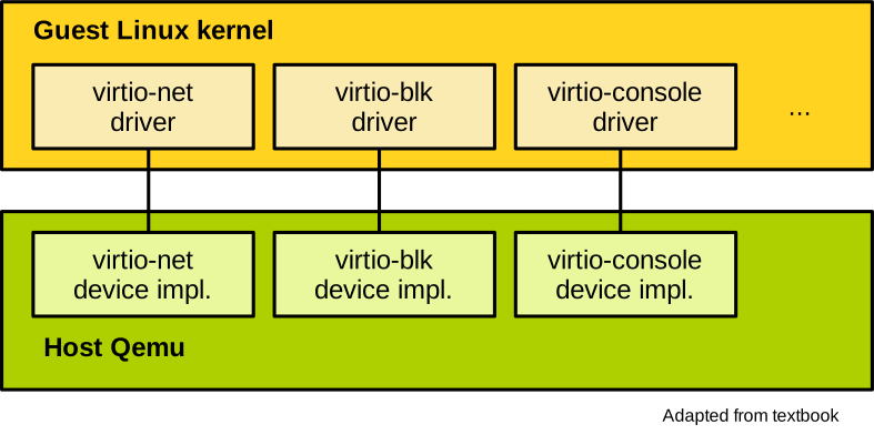
There are also virtio virtual devices that do not necessarily correspond to real physical hardware, enabling things such as memory hotplug and sharing part of the host filesystem with the VM. Because virtio is so popular, OSes such as Linux already integrate drivers for all these paravirtualised devices in the mainline kernel.
Hardware Support for I/O Virtualisation
Because full device emulation is slow, and device paravirtualisation sacrifices equivalence, there are also hardware technologies that were developed to support I/O virtualisation. A first and rather simple solution was to give a VM direct access to a device, bypassing the hypervisor. This is called direct device assignment, and it gives a VM full and exclusive access to a device:
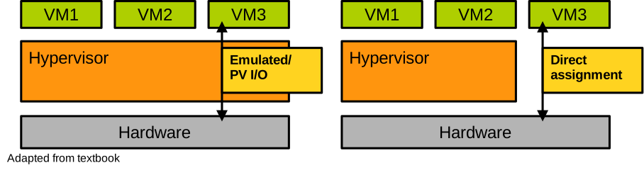
This is great from the performance and equivalence point of view, but it creates two obvious issues. First, regarding security: because the hypervisor is no longer involved, the VM can freely control the device, and in particular it can configure it to DMA anywhere in physical memory. This is a clear breach of the safety criteria. Second, in terms of scalability, each device can only be used by a single VM, so it is not very practical.
The IOMMU
The aforementioned security problem with direct device assignment is due to the fact that DMA bypasses the MMU and operates directly on physical memory. The VM controlling the device can then read from or write to anywhere in physical memory, including the areas allocated to other VMs or to the hypervisor. The VM can also force the device to trigger arbitrary interrupt vectors and can possibly inject interrupts into the host or other VMs.
The solution to these problems is the IOMMU. It is a piece of hardware on the CPU that contains mainly two technologies. First, the ability to enforce the permissions set by page tables and extended page tables on DMA requests. This way we can make sure that a VM with direct device assignment can only access the memory it is allocated. Second, the interrupt remapping engine routes all interrupts from a given device to the VM which has direct access to that device. This prevents interrupt injection attacks.
SR-IOV
A second technology is SR-IOV, which stands for single-root I/O virtualisation. It tackles the scalability issue. A device supporting SR-IOV can present several instances of itself, and each instance can be directly assigned to a VM. Doing so, the hardware virtualises and multiplexes itself. A device has one physical function which is controlled by the hypervisor, and that allows it to create several virtual functions, each representing a virtualised instance of the device directly assigned to a VM. An example of an SR-IOV-enabled network card is illustrated here, with a physical function controlled by the hypervisor, and two virtual functions, each assigned directly to a different virtual machine:
Today’s modern SR-IOV devices can create thousands of virtual functions. M
Lightweight Virtualisation
You can access the slides 🖼️ for this lecture.
Motivation
Imagine a company wishes to run a website and does not want to leave a local machine up and running 24/7, so they decide to rent a virtual machine in the cloud. They choose a cloud provider, say AWS, and select a Linux distribution to install on their VM, for example Ubuntu. So inside their VM the web server, such as Apache, is installed, along with its library dependencies, such as Perl and libssl. When Apache runs, all this software makes use of a subset of the services offered by this massive guest kernel, namely Linux. The setup we just described can be illustrated as follows:
In this illustration, what really needs to run is in the blue boxes: the web server, its dependencies, and the subset of kernel features it requires, that’s it. All the grey areas are installed and maybe even running but are not needed. We call this software bloat, and it is a genuine concern.
Indeed, software bloat first leads to an increased attack surface: all the software installed in the Linux distribution, and the background programs running—much of which you do not really need—represent potential targets for an attacker to take over as a first step toward attacking your environment. Probabilistically, the more software you run, the higher the chance that a vulnerability is present somewhere. Second, software bloat represents additional costs. The tenant of the VM is paying the cloud provider for the disk, memory, and CPU cycles used to store and run software they do not even need. Third, for a fixed budget, software bloat also causes performance loss, because all these memory and CPU cycles are not used to run what really needs to run, which is your web server.
Definition
Lightweight virtualisation tackles this issue by providing the following properties, compared to traditional virtual machines:
- Lower memory footprint, in the order of kilobytes to a few megabytes of system software overhead for each virtualised instance, compared to hundreds of megabytes or gigabytes of memory consumption for traditional VMs.
- Fast boot times in microseconds or milliseconds, compared to seconds or minutes for traditional VMs.
- Lower disk footprint, once again we are talking about a few kilobytes or megabytes.
Obviously, these metrics concern the per-VM systems software, in particular the operating system. The part of the initialisation time and memory/disk footprint that relates to an application will stay the same whether it runs in a lightweight or in a traditional VM.
Today there are three modern technologies that enable achieving these lightweightness objectives. First, stripped-down Linux VMs, called micro-VMs. These can be quite minimalist, but there are two technologies that take things one step further in terms of lightweightness: containers and unikernels. We will focus on containers and unikernels here; if you want to explore micro-VMs on your own, you can check out, for example, Firecracker.
Containers
Presentation
Containers are a process-based sandboxing technology, enforced by the operating system. A container management stack differs significantly from a system-level VM-based one:
Unlike a traditional virtual machine, a container is a process or a group of processes for which the OS restricts the visibility of system resources. This way the software running in the container is sandboxed, and it also feels as though it is running alone in the system, like in a virtual machine.
The resources whose visibility can be reduced and changed for the container are the filesystem, the system’s users, visible PIDs, IPCs, system clocks, among others. The OS can also control the allocation of certain resources to the container, including CPU scheduling cycles, available memory, and usable disk and network bandwidth, among others.
Conceptually, by reducing or changing the visibility of resources, and limiting their allocation to a process or a group of processes, containers achieve the same isolation goals as a virtual machine, without the need for a hypervisor and a system-level VM. This is much lighter than using a traditional virtual machine. The boot time is that of spawning a process, a few microseconds, and the memory footprint is close to zero. Still, containers are not perfect, and as we will see they suffer from significant security concerns.
Use Cases
Containers are useful in most scenarios where virtualisation is beneficial. They are extensively used in software development, where they allow setting up a homogeneous environment in which to develop, build, and test an application, shared by the entire development and testing team. Containers can also be used for deployment, as they represent a lightweight way to package an application together with all of its dependencies. Docker is a prime example of a container engine used extensively in software development:

Because they are so lightweight, containers can replace traditional VMs for many aspects of the cloud that require very quick initialisation and execution of a particular task. Services such as Gmail or Facebook make extensive use of containers for such tasks. You may also have heard of AWS Lambda, which provides serverless computing services. With the serverless paradigm, the developer programs cloud machines with small stateless functions executed on demand when certain events happen, for example when a user visits a web page. These functions generally run within containers.

Namespaces and Control Groups
Containers are enabled by two key technologies in Linux, which restrict the view and usage of resources for processes: namespaces and control groups.
Namespaces restrict the view of the following system resources from the container:
- Filesystems and mount points: a container is generally given its own root filesystem from a base image, and it cannot access the host’s filesystem.
- Network stack: a container also has its own state of the network stack, including its own IP, with a virtual bridged and routed network.
- Processes: PIDs and IPCs: a container also has its own isolated set of PIDs, one for each process it runs. It cannot see or communicate with external processes.
- Host and domain name: a container can set the host name, which is the machine’s name, to something different from what the host sees. The same applies to the domain name.
- User IDs: usernames and IDs can also be different within the container, compared to those on the host. In most scenarios a user will simply take on the identity of root within the container.
Control groups restrict a container’s usage and allocation of the following system resources:
- Memory: one can set the maximum amount of memory and swap a container can use.
- CPU: the CPU usage of a container can be rate-limited, for example the container can be allocated 1.5 CPUs. Which CPU (core) a container can run on can also be restricted, and so can the scheduler’s quotas for the container.
- Devices: a container can also be restricted to seeing only certain devices.
- Block and network I/O: a container’s disk and network throughput can be rate-limited.
Containers vs. VMs
If we list the respective benefits of containers versus traditional virtual machines, we get the following:
| Containers | VMs |
|---|---|
| Low memory/disk usage | OS diversity |
| Fast boot times | Kernel version |
| High density per host | Performance isolation |
| Nesting | Security |
Containers are very lightweight, meaning they have low memory and disk usage and very fast boot times. Their lightweightness allows creating a very high number of containers on a single machine; it is not uncommon to run hundreds or even thousands of containers on a host. Nested virtualisation is also easy with containers; in other words, it is simple to create a container within a container. Regarding virtual machines, they are still useful when one wants to run an operating system other than Linux—something that is difficult to do efficiently with containers because they rely on the namespaces and control groups technologies available only on Linux. Several studies have also shown that performance isolation is stronger with VMs than with containers, meaning it is more difficult for a malicious VM to steal resources by abusing them. Finally, the degree of isolation of the sandboxing enforced by virtual machines is considered much stronger than that of containers.
Containers and Security
To understand why the isolation of VM environments is considered stronger than that of containers, let us consider both setups:
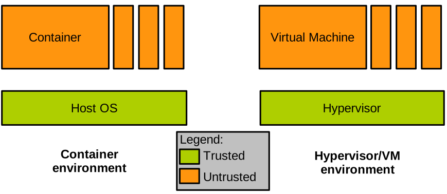
We have a container environment on the left, with several containers running on top of the OS kernel. And on the right a VM environment, with several VMs running on top of a hypervisor. If we place ourselves in the shoes of the cloud provider, and reason about what we trust and what we do not trust in such a setup, we shall conclude that the virtualisation layer is trusted, that is the OS for the container environment, and the hypervisor for the VM one. The instances of either containers or virtual machines are obviously untrusted; who knows who the tenants are and what they run in their VMs/containers.
As the provider of virtualised environments, the kind of attack we are most concerned about is often the following:
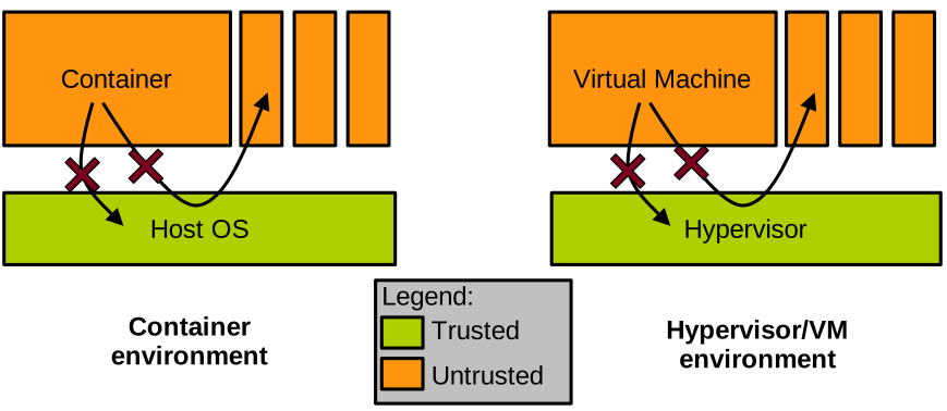
One of the containers or VMs is malicious, and tries to perform an escape attack, that is, to gain access to the virtualisation layer’s memory, or to the memory allocated to other containers or VMs. As we have seen in the past, hardware-enforced isolation mechanisms such as the page tables or extended page tables will prevent direct access from the malicious entity to other VMs or containers. The real threat lies in the virtualisation layer, which can be invoked by the malicious VM or container. If such an invocation manages to trigger a bug in the virtualisation layer, the isolation may be broken and the attacker could access the virtualisation layer’s, or another container’s or VM’s, memory.
It is quite important to determine how complex this interface between what we trust and what we do not trust is in both cases. The reason is that how complex the interface is translates directly into how hard it is to secure this interface and make sure there are no bugs.
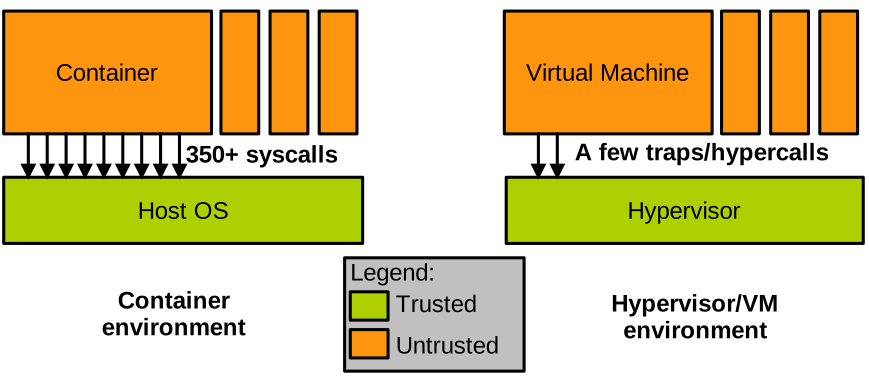
In the case of containers, that interface is unfortunately very complex: it is the system call interface, which comprises hundreds of system calls, some of them like ioctl presenting thousands of sub-functions.
There is no way we can guarantee that the implementation of all these system calls is bug-free.
In fact, automated vulnerability detection systems regularly find bugs in that interface.
Conversely, the interface between a VM and the hypervisor managing it is much simpler: it is just a few traps.
In that context, the isolation between containers is not considered as strong as that between VMs, because of the complexity of the interface between containers and the privileged layer, the OS kernel. To illustrate this point, note that many actors running containers in production actually run containers within virtual machines, to benefit from their strong isolation. These approaches try to reduce the memory footprint and boot times of Linux VMs as much as possible, creating what they call micro-VMs; however, this still negates most of the lightweightness benefits of containers. An example of such technology is Firecracker.
Unikernels
Presentation
We have seen that traditional VMs are heavyweight but secure, and that containers are lightweight but insecure. Can we get both the lightweightness benefits of containers, combined with the security benefits of virtual machines, into a single virtualised solution? Unikernels are a relatively new operating system model that aims to answer that question.
Recall our motivational example from earlier, presenting the software bloat that occurs in many situations when using traditional VMs. Using unikernels we would address the problem as follows:
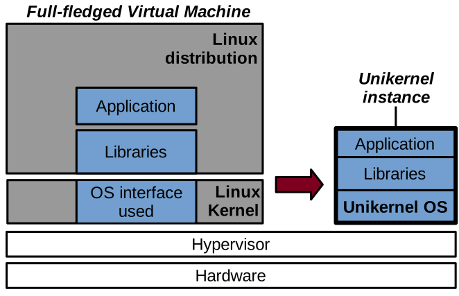
With a unikernel we compile an application’s code, as well as all of its dependencies, together with a very small operating system layer into a static binary that merges the application and the operating system. This binary can be run as a kernel, in a virtual machine, on top of a hypervisor.
A unikernel instance is single-purpose and it runs a single application. To run multiple applications, one needs to run multiple unikernel instances. A unikernel instance is also a single-process virtual machine, and once again, to run a multi-process application, several unikernel instances must generally be run. Still, several unikernel models can run on multicore CPUs and leverage parallelism/concurrency with threads. Finally, as already mentioned, a unikernel instance runs a single binary, containing the application, its dependencies, and the kernel. All of this code runs within a single address space, and there is no user/kernel protection. This is because there is only one application running in a unikernel instance, and the isolation between applications is already enforced by running them as separate unikernel instances.
The unikernel model was originally proposed in this seminal paper in 2013:
Madhavapeddy et al., Unikernels: Library Operating Systems for the Cloud, ASPLOS’13
Benefits & Application Domains
With that model, unikernels present a series of benefits. First, it is a form of lightweight virtualisation. Because a unikernel instance only runs the code absolutely necessary for the application in question, and because the OS layer is so small, we get similar benefits to those of containers in terms of low memory/disk footprint and fast boot times. Second, because they run as virtual machines, unikernels are well isolated and considered a secure alternative to containers in many scenarios. Third, the OS layer within a unikernel instance can be specialised towards the application it runs: specialised kernel subsystems can bring higher performance, or lower memory footprint and power consumption, for a particular application scenario. Finally, because a unikernel operating system is so small and simple, it does not get in the way of the application’s performance as much as larger operating systems such as Linux. This translates into increased performance for certain applications. Another noteworthy point regarding performance is the system call latency: with unikernels, because there is no user/kernel isolation, system calls are simple function calls, which makes them much faster.
Just to illustrate the unikernel performance benefits that come from their low-latency system calls, consider these results:
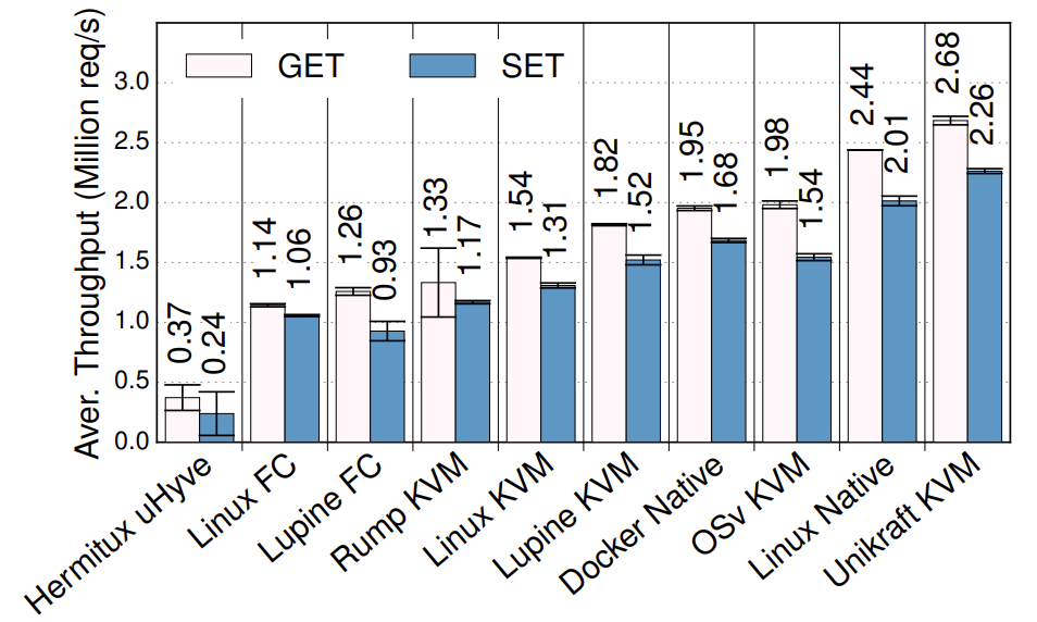
Redis throughput under various setups (higher is better)
This graph is taken from the Unikraft paper:
S. Kuenzer et al., Unikraft: Fast, Specialized Unikernels the Easy Way, EuroSys’21
The graph shows the throughput of Redis, which is a very popular key-value store, in millions of requests per second. There are various setups on the x-axis, including different unikernels, as well as vanilla Linux. As you can see, Unikraft is the fastest solution: even though it runs virtualised on top of QEMU/KVM, it is still a bit faster than non-virtualised Linux, and also much faster than Linux in a VM. Feel free to check out the paper for a more detailed performance evaluation.
Given these benefits, unikernels have plenty of application domains. We motivated them with cloud environments such as server or microservice software. But they have also been explored in the domains of embedded virtualisation, edge computing and IoT, network function virtualisation, high-performance computing, and various security-critical domains such as VM introspection, malware analysis, and secure desktop environments. Still, an important point to note is that most unikernels are still at the stage of research prototypes. This is different from containers, which, as you may know, are a production-ready technology.
Unikernel Projects

A few examples of unikernel projects are listed below. Some of these are relatively unstable and poorly maintained academic research artefacts. The most mature project, and the one closest to production-ready status, is Unikraft.
Unikernels can be classified based on the target languages for the supported applications:
- Pure memory-safe languages (OCaml, Erlang, Haskell): MirageOS, LING, HalVM
- C/C++, semi-POSIX API: Unikraft, HermiTux, HermitCore, OSv, Rumprun, Lupine
- Rust/Go: Hermit, Clive
- More: https://unikernelalliance.org/projects/
Compatibility Aspects
Although they present desirable security and lightweightness benefits, unikernels also suffer from an important drawback that stems from their custom OS nature: a lack of compatibility with existing software and, to a lesser extent, hardware. On the hardware side, it is not possible for unikernel projects to integrate the large number of drivers supported by popular operating systems such as Windows or Linux. Still, using the split driver model (frontend/backend) that we saw is common in virtualised environments, a unikernel supporting popular paravirtualised (e.g., Virtio) I/O frontend drivers and running alongside a host operating system such as Linux will be compatible with numerous I/O devices. The real compatibility problem of unikernels rather lies on the software side.
One of the reasons unikernels are not particularly popular today, despite being around for more than a decade, is that it is hard to run existing applications on top of them. Most unikernels require access to an application’s source in order to compile it with the unikernel OS, so in scenarios where the source is not available for a given application (e.g., proprietary software), a unikernel cannot be created. Even when the source is available, as we have seen previously, most unikernel models support only one or a few programming languages, which limits compatibility.
Many applications will also require specific OS features available under Linux or Windows, but unsupported by most unikernel models. Porting is thus required: one can try to adapt an application to work on top of a unikernel model, or to enhance the unikernel model so that it provides the features required by the application. Often, porting involves doing a bit of both: it is a time-consuming task that requires expertise in both the application to be ported and the unikernel model to use, which discourages many prospective users.
Since this problem was identified, several research efforts have attempted to address the compatibility issues of unikernels. The main idea is to require as few modifications, and as little effort, as possible to execute, as a unikernel, an application that already builds for and runs on top of a popular operating system such as Linux. Compatibility can be achieved at various levels, from the weakest to the strongest:
- Source-level compatible unikernels (e.g., HermitCore, Rumprun): these require recompiling an application’s code with a custom C standard library and the unikernel kernel. This is a relatively weak form of compatibility, as the C standard library is not the only interface to the kernel in many applications. This approach also still requires recompilation and access to the source.
- C standard library-level binary-compatible unikernels (e.g., OSv, Lupine): these interface with an application at runtime through a custom C standard library, similarly to how shared libraries are loaded at runtime. These approaches may sometimes avoid recompilation, but are still limited to programs that request OS services only through the C standard library.
- System call-level binary-compatible unikernels (e.g., HermiTux, Unikraft): this is the strongest form of compatibility, targeting the standard application/OS interface: the unikernel OS hooks into the system calls made by an application compiled for a popular operating system (e.g., Linux) and emulates that OS behaviour. Such compatibility at the system call level allows running unmodified Linux applications as unikernels without access to the source or recompiling.
For more information on the topic of unikernels and application compatibility, check out this paper:
Olivier et al., A Binary-Compatible Unikernel, VEE’19
Virtualisation: Further Readings
System-level Virtualisation
- Popek and Goldberg, Formal Requirements for Virtualizable Third Generation Architectures. The foundational paper upon which the “Theory of Virtualisation” part of the unit is built.
- Barham et al., Xen and the Art of Virtualization. Xen’s paper, seminal work on paravirtualisation.
- Bugnion et al., Disco: Running Commodity Operating Systems on Scalable Multiprocessors. Another seminal work.
- Clark et al., Live Migration of Virtual Machines. Seminal work on VM migration.
- Kivity et al., kvm: the Linux Virtual Machine Monitor. KVM’s paper.
- (book) Bugnion et al., Hardware and Software Support for Virtualization. Book which inspired much of this week’s content.
Containers
- Banga et al., Resource Containers: A New Facility for Resource Management in Server Systems.
- Soltesz et al., Container-based Operating System Virtualization: A Scalable, High-performance Alternative to Hypervisors.
- Heo, Control Group v2.
- Kerrisk, Namespaces in operation.
Unikernels
- Madhavapeddy et al., Unikernels: Library Operating Systems for the Cloud. Seminal unikernel paper.
- Kivity et al., OSv—Optimizing the Operating System for Virtual Machines. OSv’s paper.
- Kuenzer et al., Unikraft: fast, specialized unikernels the easy way. Unikraft’s paper.
- Olivier et al., A Binary-Compatible Unikernel. Pierre’s work on unikernels and application compatibility.
- More unikernel papers here.